 (1)
摘要 为了获取光纤复合架空地线(OPGW)的覆冰判据及其覆冰厚度的监测方法,该文首先采用WAVE法模拟真实环境温度随时间的变化,建立了OPGW覆冰时的三维温度场模型,并在人工气候室中基于布里渊光时域反射仪(BOTDR)开展了覆冰试验,验证了模型的有效性,同时在仿真和试验中验证了线路温度的滞后特征。其次,提出了光纤与环境温度曲线间的相位差、升温速度变化率与波动幅值变化率三个温度滞后特征量,基于验证后的温度场模型建模研究获得了不同覆冰厚度下三个特征量的数值,并通过拟合分别给出了对应的覆冰厚度估算公式。最后,建模研究了环境温度变化与光纤温度测量误差对三个特征量的影响,进一步获得了含噪声的光纤温度数据,并基于该数据研究了噪声对上述三个公式计算准确性的影响,同时对不同公式受噪声影响的程度进行了对比分析。结果表明:环境温度均值、波动幅值对三个特征量的影响均较小,可以忽略其对覆冰厚度估算的影响。光纤温度测量误差对升温速度变化率与波动幅值变化率的影响较大,而对相位差影响较小。基于温度曲线相位差的覆冰估算准确性最优,若温度滞后特征量选择不合理,覆冰厚度估算误差最高可扩大8倍。
关键词:光纤复合架空地线(OPGW) 布里渊光时域反射(BOTDR) 覆冰判据 温度滞后特征量 覆冰厚度监测
输电线路覆冰事故[1-2]是威胁电力系统安全运行的主要因素之一,对其进行有效防控已成为保障电网稳定运行的重要课题[3-6]。传统输电线路覆冰在线监测系统多采用点式传感器[7-8],存在安装复杂、监测范围有限等问题,如果要实现全面监测,可能需要布设数千台点式传感器。相比之下,分布式光纤传感(Distributed Optical Fiber Sensing, DOFS)技术[9-11]具有诸多优势,包括监测距离远、测量精度高、受电磁噪声影响小等[12-13]。更重要的是,对于光纤复合架空地线(Optical Fiber Composite Overhead Ground Wire, OPGW),不需要增设额外的传感器[14]。因此,DOFS技术作为一种新兴的低成本传感技术,在输电线路覆冰监测领域得到了广泛应用[15-17]。
布里渊光时域反射仪(Brillouin Optical Time Domain Reflectometer, BOTDR)由于其单端测量和对温度敏感等优势[18-19],常被用于工程中监测OPGW覆冰时的温度状态。近年来,基于BOTDR的输电线路覆冰监测技术多利用覆冰段与未覆冰段不同的温度变化特征来监测覆冰状态。当环境温度以线性模式变化时,该方法的有效性已得到初步验证。吴念等[20]搭建了覆冰OPGW二维仿真模型,发现环境温度线性下降时覆冰段温度整体变化较未覆冰段更小;覃兆宇等[21]也采用类似模型模拟了环境温度线性上升或下降的情况,验证了覆冰段对环境温度变化敏感度比未覆冰段较低的结论;Sun Jinxiang等[22]采用二维OPGW模型与试验验证相结合的方式,验证了环境温度线性变化下覆冰段相对于未覆冰段不同的温度变化特性,并发现随着覆冰厚度增加,二者差距越来越明显;Zou Xiaoming等[23]建立了OPGW覆冰时径向和轴向两个二维温度场模型,基于该模型研究了环境温度线性变化时光纤温度随时间的变化,给出了基于覆冰段与未覆冰段间光纤温差的覆冰厚度估算公式。
然而,实际环境温度通常随时间呈非线性变化,此时基于环境温度线性变化的上述研究结果无法直接应用,这就给在实际中的应用引入了不确定性。为了提高可靠性,文献[24]采用正弦函数模拟环境温度-时间变化曲线,发现了输电线路温度相对于环境温度的滞后现象,提出利用光纤与环境温度曲线间的峰值时间差来计算相位差,并基于相位差监测覆冰厚度。然而,文献[24]缺乏试验验证。此外,覆冰段光纤温度曲线相对于环境温度的滞后现象可能存在多个特征量。这些特征量用于覆冰监测时的有效性有待进一步比较,同时也需要确定最佳特征量。以上研究均未见文献报道。
为此,本文通过仿真与试验,对比分析了光纤与环境温度曲线间的相位差、升温速度变化率与波动幅值变化率这三个温度滞后特征量,并给出了基于三个温度滞后特征量的OPGW覆冰厚度估算公式。进一步地,通过仿真与试验对三个特征量的覆冰厚度监测方法进行对比验证,最终确定了最优的温度滞后特征量。
现有覆冰线路的热力学模型研究以二维模型为主[20-23],为了更好地模拟线路与环境间的热力学关系,同时克服线性变化或恒定温度[25]的不足,本文建立了正弦环境温度激励下OPGW覆冰时的三维温度场模型,并在人工气候室内进行验证。
1.1.1 OPGW覆冰热力学分析
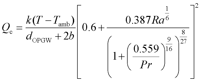
太阳辐射、空气绕流导线的自然对流散热和导线自身向环境的辐射散热是引起覆冰OPGW温度变化的主要原因[22]。设Qs、Qc和Qr分别为太阳辐射、空气绕流导线的自然对流散热和导线自身向环境的辐射散热,其表达式分别[20-22]为
(1)
 (2)
 (3)
式中,α为吸热系数;J为太阳辐射率;dOPGW为OPGW线路直径;b为覆冰厚度;k为空气的导热系数;T为线路温度,℃;Tamb为环境温度,℃;Ra为空气的瑞利数;Pr为空气的普朗特数;εs为表面辐射系数;σ为斯忒藩-玻耳兹曼常数。
在不考虑融冰对线路温度影响的情况下,可采用瞬态热传导方程研究线路在不同环境温度和不同覆冰厚度下温度随时间的变化情况,线路覆冰和未覆冰时的瞬态传热方程分别为
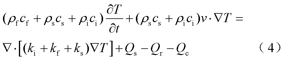
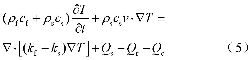
式中,ρf、ρs和ρi分别为光纤、钢和冰的密度;cf、cs和ci分别为光纤、钢和冰的比热容;t为时间;v为风速;kf、ks和ki分别为光纤、钢和冰的导热系数。
由式(4)和式(5)可知,除了太阳辐射、对流散热和辐射散热的影响外,空气的比热容与冰的比热容不同,导致覆冰段线路的等效比热容不同,这也是引起覆冰段与未覆冰段线路温度变化不同的原因。
1.1.2 应变对光纤温度的干扰
布里渊频移受光纤温度和施加在光纤上的应变的影响,表示为
 (6)
式中, 为布里渊频移;
 和
 分别为应变和温度变化量;
 和
 分别为初始应变和初始温度;
 和
 分别为布里渊频移的温度和应变的敏感系数。
覆冰初期所造成的拉力较小,不足以完全消耗光纤余长[26],可以认为光纤所受应变基本不变,应变对布里渊频移的影响可以忽略,光纤沿线的布里渊频移只与沿线温度有关。当施加在光纤上的应变不变时,布里渊频移可以表示为温度的函数,即
 (7)
当覆冰厚度较大时,光纤余长被完全消耗,布里渊频移同时受光纤温度和应变的影响,覆冰应变会导致布里渊频移和解调得到的温度随时间变化的曲线整体上移。但这种整体的变化并不会影响后文中的相位差、升温速度变化率和波动幅值变化率,所以即使存在应变的干扰,也不会影响本文方法的准确性。
1.1.3 OPGW覆冰三维温度场模型的建立
在COMSOL Multiphysics中建立覆冰OPGW温度场模型。模型中OPGW型号为OPGW-24B1-155,考虑实际情况对其进行简化,得到简化OPGW模型截面示意图如图1所示。忽略铝包钢线之间的缝隙和光纤间的填充油膏,将光纤和铝包钢线分别等效为整体[27-28]。认为材料各向同性,各部分的导热系数不变。后文1.2节中仿真和试验结果的对比验证了上述简化的合理性。三维覆冰OPGW模型参考后续试验中的参数,线路长4 m,覆冰段位于线路上2~3 m之间,假设冰层均匀覆盖线路,建立三维覆冰OPGW模型如图2所示。仿真计算中涉及的结构参数和材料属性见表1。
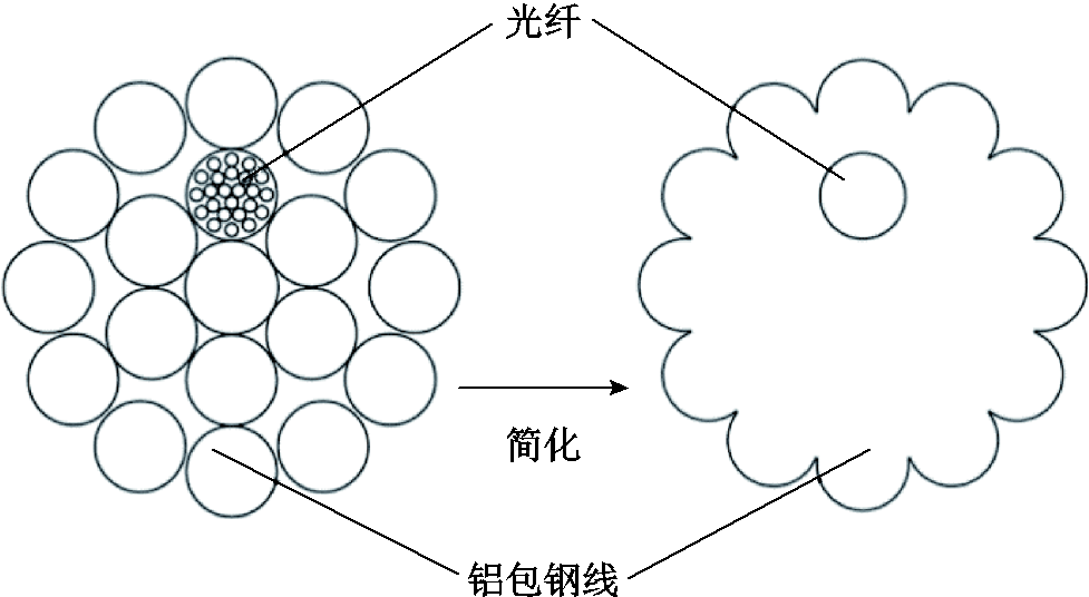
图1 简化OPGW模型截面示意图
Fig.1 Simplified section diagram of OPGW model
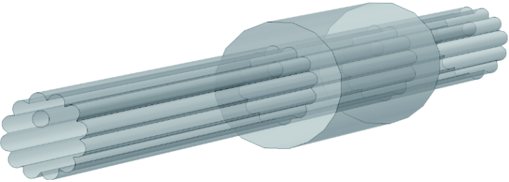
图2 三维覆冰OPGW模型
Fig.2 Three dimensional ice covered OPGW model
表1 仿真计算中的结构参数和材料属性
Tab.1 Structural parameters and material properties in simulation calculations

参数数值参数数值 b/mm5cs/[J/(kg∙K)]475 ρf/(kg/m3)2 203ci/[J/(kg∙K)]2 100 ρs/(kg/m3)7 850kf/[W/(m∙K)]1.38 ρi/(kg/m3)900ks/[W/(m∙K)]44.5 cf/[J/(kg∙K)]703ki/[W/(m∙K)]2.24
假设覆冰厚度为5 mm,线路与环境的初始温度为-1℃,环境温度以-2℃/h的速率从-1℃降至-7℃,仿真时间为3 h。得到3 h时三维覆冰OPGW模型的温度分布如图3所示,不同时刻OPGW中光纤沿线温度变化如图4所示。
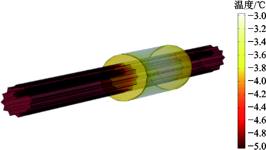
图3 三维OPGW模型的温度分布
Fig.3 Temperature distribution of three-dimensional OPGW model
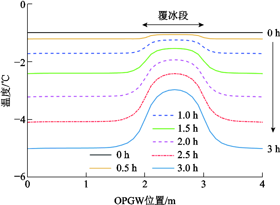
图4 三维OPGW模型中光纤温度随时间的变化
Fig.4 Change of optical fiber temperature with time in the three-dimensional OPGW model
由图4可以看出,当环境温度线性下降时,相同时刻覆冰段线路的温度相对于未覆冰段下降得更少。其原因为,一方面,线路覆冰后,冰的导热系数远小于线路的导热系数,影响了自然对流散热;另一方面,冰的比热容比标准大气压下空气的比热容大,而空气的密度较小,导致冰的体积热容远大于空气,覆冰段线路等效比热容大于未覆冰段线路。3 h时,覆冰段与未覆冰段最大温差达2.04℃。因此,当环境温度变化时,覆冰段与未覆冰段温度存在明显不同的变化特征。
为了展现更接近真实环境温度变化下覆冰段线路的温度变化特征,并对上述模型进行验证,在人工气候室(徐州市三禾自动控制设备有限公司冷库PLC工程技术研究中心)内进行了覆冰OPGW的温度测量试验,覆冰试验中的OPGW如图5所示。OPGW线路长度约为4 m,覆冰段位于线路上2~3 m之间,覆冰厚度约为5 mm,共开展了2次试验。测温试验于线路覆冰结束后进行,先将环境温度升高1 h,再降低1 h,然后重复上述过程一次。通过温度传感器直接测量环境温度的变化。利用BOTDR(型号:6419A,中电科思仪科技股份有限公司)测量光纤复合线路中的布里渊光谱,计算相应的布里渊频移值。布里渊频移与光纤温度和施加在光纤上的应变呈线性关系,试验中应变随时间变化对布里渊频移的影响可以忽略,认为布里渊频移仅与光纤温度有关。由预试验得到布里渊频移-温度系数为1.12 MHz/℃,进而得到试验中光纤温度随时间的变化,如图6所示。根据试验参数建立了相应的覆冰OPGW仿真模型,仿真结果如图7所示。需要注意的是,由于光纤与环境温度曲线之间存在滞后,光纤复合线路覆冰段和未覆冰段的光纤初始温度由与上述模型类似的温度场模型确定。
由图6和图7可知,覆冰段、未覆冰段的光纤温度曲线与环境温度曲线之间存在明显的滞后现象。试验结果与仿真结果基本吻合,验证了本文建立温度场模型的正确性。

图5 覆冰试验中的OPGW
Fig.5 OPGW in icing experiment
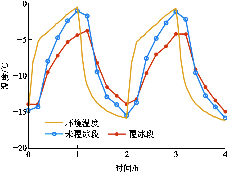
图6 5 mm覆冰时光纤与环境温度随时间的变化(试验)
Fig.6 The variation of fiber optic and ambient temperature over time when ice thickness is 5 mm (experiment)
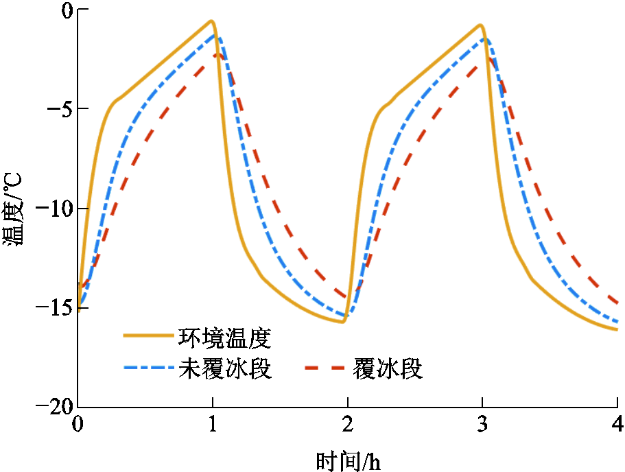
图7 5 mm覆冰时光纤与环境温度随时间的变化(仿真)
Fig.7 The variation of fiber optic and ambient temperature over time when ice thickness is 5 mm (simulation)
根据大量统计数据研究,日气温变化可用多种函数方法进行模拟。WAVE法因其对特定地区的假设和校准因素最少,被认为具有最好的日气温变化模拟效果[29],其表达式为
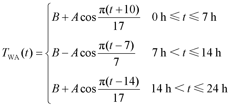 (8)
式中,TWA(t)为由WAVE法表示的环境温度;A和B分别为环境温度的波动幅度和平均值,℃。
环境温度变化采用WAVE法模拟。令A=5℃,B=-5℃,覆冰厚度为5、10 mm,仿真时间为168 h。如无特殊说明,线路初始温度与环境温度一致,日出时间为7:00,日落时间为18:00,太阳辐照度为200 W/m2[22],其余参数均与1.2节中保持一致。当覆冰厚度分别为5、10 mm时,计算得到的线路覆冰段和未覆冰段光纤温度曲线如图8和图9所示。
由图8和图9可知,覆冰段和未覆冰段光纤温度曲线呈现与环境温度相似的周期性变化。但是与环境温度曲线相比,存在明显的滞后现象。这种滞后现象一方面表现为温度曲线整体在时间轴上的向后偏移,另一方面表现为温度变化速度变慢,同时也表现为温度曲线在温度波动范围上的缩小。若能定量描述这种由线路覆冰引起的滞后现象,就有望基于滞后特征量对线路的覆冰状况进行评估。
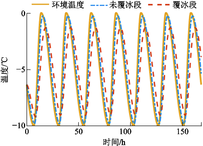
图8 5 mm覆冰时光纤与环境温度随时间的变化(仿真时间168 h)
Fig.8 The variation of optical fiber and environmental temperature over time when covered with 5 mm ice (simulation time 168 hours)
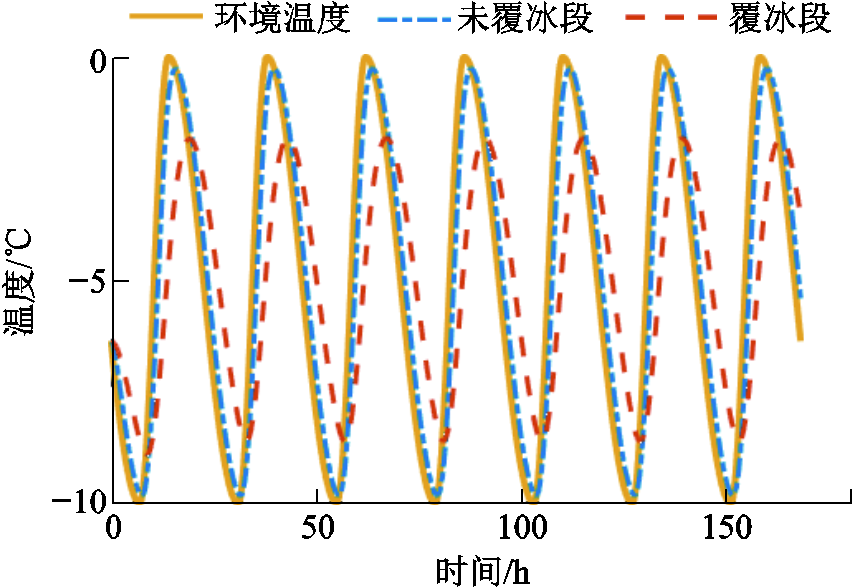
图9 10 mm覆冰时光纤与环境温度随时间的变化(仿真时间168 h)
Fig.9 The variation of optical fiber and environmental temperature over time when covered with 10 mm ice (simulation time 168 hours)
为了对该滞后现象进行定量描述,本文提出光纤与环境温度曲线间的相位差、升温速度变化率与波动幅值变化率这三个特征量。考虑到实际情况,对于仿真时长大于24 h的情况,三个温度滞后特征量均采用最后24 h的数据进行计算。
温度曲线相位差通过离散傅里叶变换(Discrete Fourier Transform, DFT)进行求解,计算过程采用快速傅里叶变换(Fast Fourier Transform, FFT)算法提升计算效率。设TA(n)和TI(n)分别为环境温度序列与覆冰段光纤温度序列,0≤n≤N-1,分别对它们进行DFT,得到
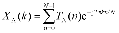 (9)
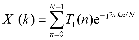 (10)
式中,k为基频(周期为24 h)对应的序号;N为测量点数。
根据DFT结果可计算两条温度曲线之间的相位差φ(°),有
 (11)
式中,arg[X]为复数X的相位。
温度曲线升温速度变化率rv与波动幅值变化率ra的计算式分别为
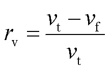 (12)
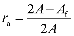 (13)
式中,vt为环境温度曲线在24 h内升温速度的最大值;vf为覆冰段光纤温度曲线在24 h内升温速度的最大值;Af为在24 h内覆冰段光纤温度曲线的峰峰值,℃。
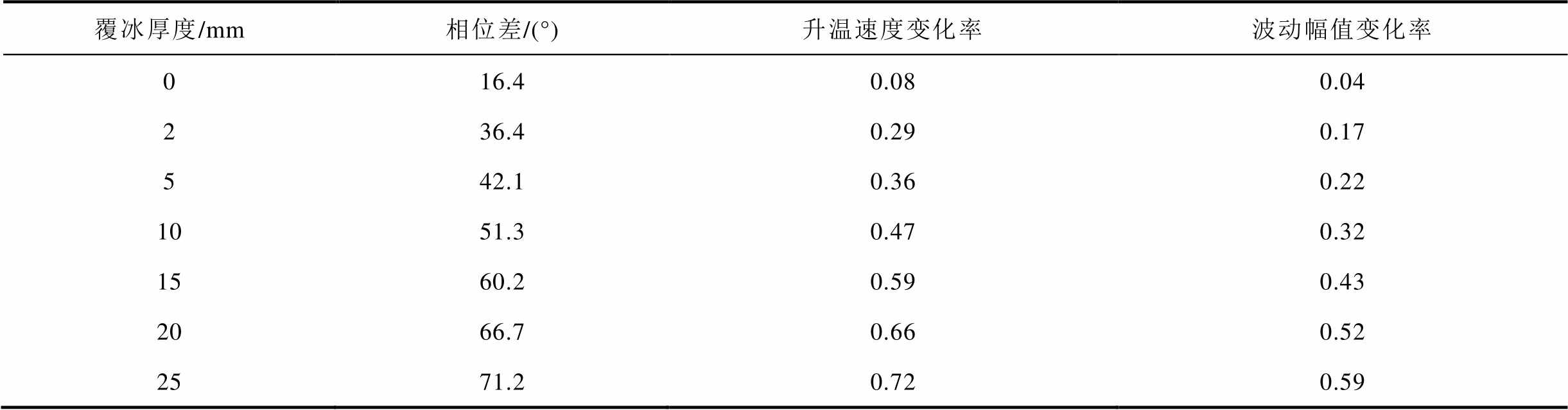
环境温度变化采用WAVE法模拟。令A=5℃,B=-5℃,覆冰厚度分别为0、2、5、10、15、20、25 mm,仿真时间为168 h,其余参数均与1.2节中保持一致。得到不同覆冰厚度时覆冰段光纤温度如图10所示,计算得到的三个特征量见表2。由图10和表2可知,当覆冰厚度增加时,覆冰段光纤温度曲线的滞后程度随之增加,同时相位差、升温速率变化率与波动幅值变化率均随之增加。可见覆冰后光纤温度存在滞后情况,且三个特征量均能有效地反映不同覆冰状况下线路温度滞后特征的变化。

图10 不同覆冰厚度时覆冰段光纤温度
Fig.10 Optical fiber temperature in the ice covered section at different ice thicknesses
根据表2可以得到基于三个特征量的覆冰厚度估算公式分别如式(14)~式(16)所示。三个公式的确定系数R2分别为0.997 3、0.996 6和0.995 6,方均根误差(Root-Mean-Square Error, RMSE)分别仅为0.449 0、0.510 2、0.577 2 mm。
表2 不同覆冰厚度下的三个特征量
Tab.2 Calculated three parameters at different ice thicknesses
覆冰厚度/mm相位差/(°)升温速度变化率波动幅值变化率 016.40.080.04 236.40.290.17 542.10.360.22 1051.30.470.32 1560.20.590.43 2066.70.660.52 2571.20.720.59
 (14)
 (15)
 (16)
式中,bc为计算得到的覆冰厚度,mm。
基于上述公式,可以根据实际测得的温度滞后特征量对线路覆冰厚度进行估算。
考虑到实际情况,本节研究环境温度均值B、环境温度波动幅值A、光纤温度的测量间隔与测量误差对不同覆冰厚度估算公式的影响。
3.1.1 环境温度均值的影响
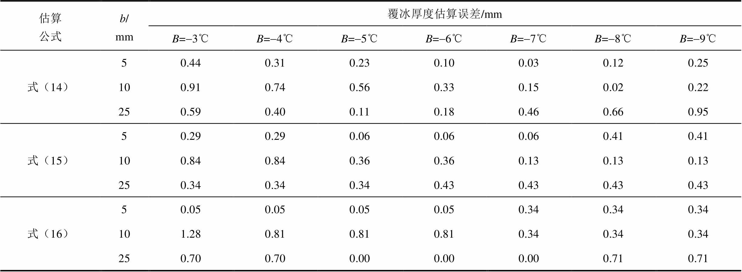
环境温度变化采用WAVE法模拟。令A=3℃,B=-3、-4、-5、-6、-7、-8、-9℃,b=5、10、25 mm,仿真时间为168 h,其余参数均与1.2节中保持一致。以b=10 mm为例,得到不同环境温度均值时覆冰段光纤温度如图11所示。计算得到的三个特征量见表3,对应的覆冰厚度估算误差见表4。

图11 不同环境温度均值时覆冰段光纤温度
Fig.11 Optical fiber temperature in the ice covered section at different average environmental temperatures
表3 环境温度均值对三个特征量计算结果的影响
Tab.3 Influence of average environmental temperature on the calculated three parameters

特征量b/mm计算结果 B=-3℃B=-4℃B=-5℃B=-6℃B=-7℃B=-8℃B=-9℃ 相位差/(°)541.742.042.242.542.843.043.3 1050.851.151.451.852.152.352.7 2570.971.171.471.772.072.272.5 升温速度变化率50.360.360.370.370.370.380.38 100.470.470.480.480.490.490.49 250.720.720.720.730.730.730.73 波动幅值变化率50.220.220.220.220.230.230.23 100.310.320.320.320.330.330.33 250.580.580.590.590.590.600.60
表4 不同环境温度均值时的覆冰厚度估算误差
Tab.4 Estimation error in ice thickness at different average environmental temperatures
估算公式b/mm覆冰厚度估算误差/mm B=-3℃B=-4℃B=-5℃B=-6℃B=-7℃B=-8℃B=-9℃ 式(14)50.440.310.230.100.030.120.25 100.910.740.560.330.150.020.22 250.590.400.110.180.460.660.95 式(15)50.290.290.060.060.060.410.41 100.840.840.360.360.130.130.13 250.340.340.340.430.430.430.43 式(16)50.050.050.050.050.340.340.34 101.280.810.810.810.340.340.34 250.700.700.000.000.000.710.71
由图11和表3、表4可知,环境温度均值对相位差、升温速度变化率与波动幅值变化率的影响较小,应用式(14)~式(16)对覆冰厚度的估算误差较小。覆冰厚度为5、10、25 mm时,式(14)对应的覆冰厚度估算误差最大分别为0.44、0.91、0.95 mm,式(15)对应的覆冰厚度估算误差最大分别为0.41、0.84、0.43 mm,式(16)对应的覆冰厚度估算误差最大分别为0.34、1.28、0.71 mm。因此,环境温度均值不是影响三个公式准确性的主要因素。
3.1.2 环境温度波动幅值的影响
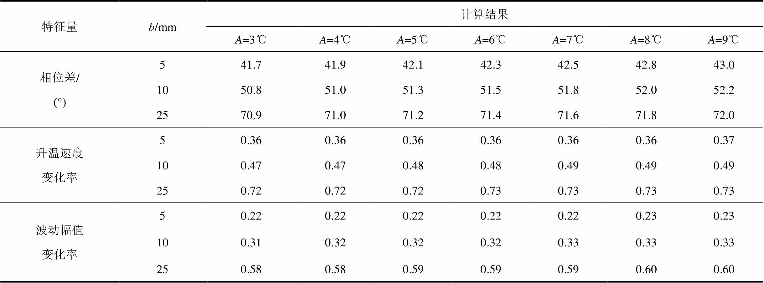
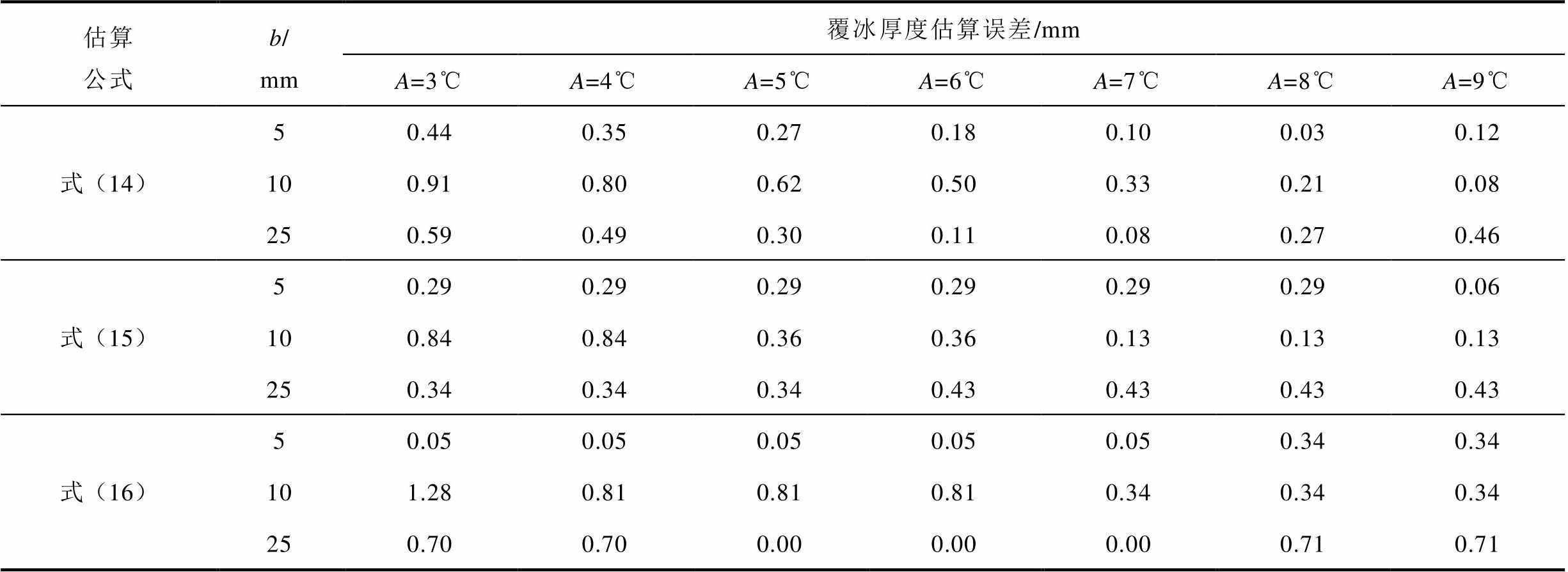
环境温度变化采用WAVE法模拟。令B=-A,A=3、4、5、6、7、8、9℃,b=5、10、25 mm,仿真时间为168 h,其余参数均与1.2节中保持一致。以b=10 mm为例,得到不同环境温度波动幅值时覆冰段光纤温度如图12所示。计算得到的三个特征量见表5,对应的覆冰厚度估算误差见表6。

图12 不同环境温度波动幅值时覆冰段光纤温度
Fig.12 Optical fiber temperature in the ice covered section at different environmental temperature fluctuation amplitudes
表5 环境温度波动幅值对三个特征量计算结果的影响
Tab.5 Influence of environmental temperature fluctuation amplitude on the calculated three parameters
特征量b/mm计算结果 A=3℃A=4℃A=5℃A=6℃A=7℃A=8℃A=9℃ 相位差/(°)541.741.942.142.342.542.843.0 1050.851.051.351.551.852.052.2 2570.971.071.271.471.671.872.0 升温速度变化率50.360.360.360.360.360.360.37 100.470.470.480.480.490.490.49 250.720.720.720.730.730.730.73 波动幅值变化率50.220.220.220.220.220.230.23 100.310.320.320.320.330.330.33 250.580.580.590.590.590.600.60
表6 不同环境温度波动幅值时的覆冰厚度估算误差
Tab.6 Estimation error in ice thickness at different environmental temperature fluctuation amplitudes
估算公式b/mm覆冰厚度估算误差/mm A=3℃A=4℃A=5℃A=6℃A=7℃A=8℃A=9℃ 式(14)50.440.350.270.180.100.030.12 100.910.800.620.500.330.210.08 250.590.490.300.110.080.270.46 式(15)50.290.290.290.290.290.290.06 100.840.840.360.360.130.130.13 250.340.340.340.430.430.430.43 式(16)50.050.050.050.050.050.340.34 101.280.810.810.810.340.340.34 250.700.700.000.000.000.710.71
由图12和表5、表6可知,环境温度波动幅值对三个特征量的影响同样较小。当覆冰厚度为5、10、25 mm时,式(14)对应的覆冰厚度估算误差最大分别为0.44、0.91、0.59 mm,式(15)对应的覆冰厚度估算误差最大分别为0.29、0.84、0.43 mm,式(16)对应的覆冰厚度估算误差最大分别为0.34、1.28、0.71 mm。因此,环境温度波动幅值同样不是影响式(14)~式(16)准确性的主要因素。
3.1.3 环境温度与覆冰厚度的影响
环境温度变化采用WAVE法模拟。为了验证环境温度与覆冰厚度共同变化下公式计算的可靠性,令B=-A,A=3、4、5、6、7、8、9℃,b=0、2、5、10、15、20、25 mm,仿真时间为168 h,其余参数均与1.2节中保持一致。根据仿真结果计算得到的相位差、升温速度变化率与波动幅值变化率见表7,对应的覆冰厚度估算误差见表8。
表7 环境温度与覆冰厚度对三个特征量计算结果的影响
Tab.7 Influence of environmental temperature and ice thickness on the calculated three parameters
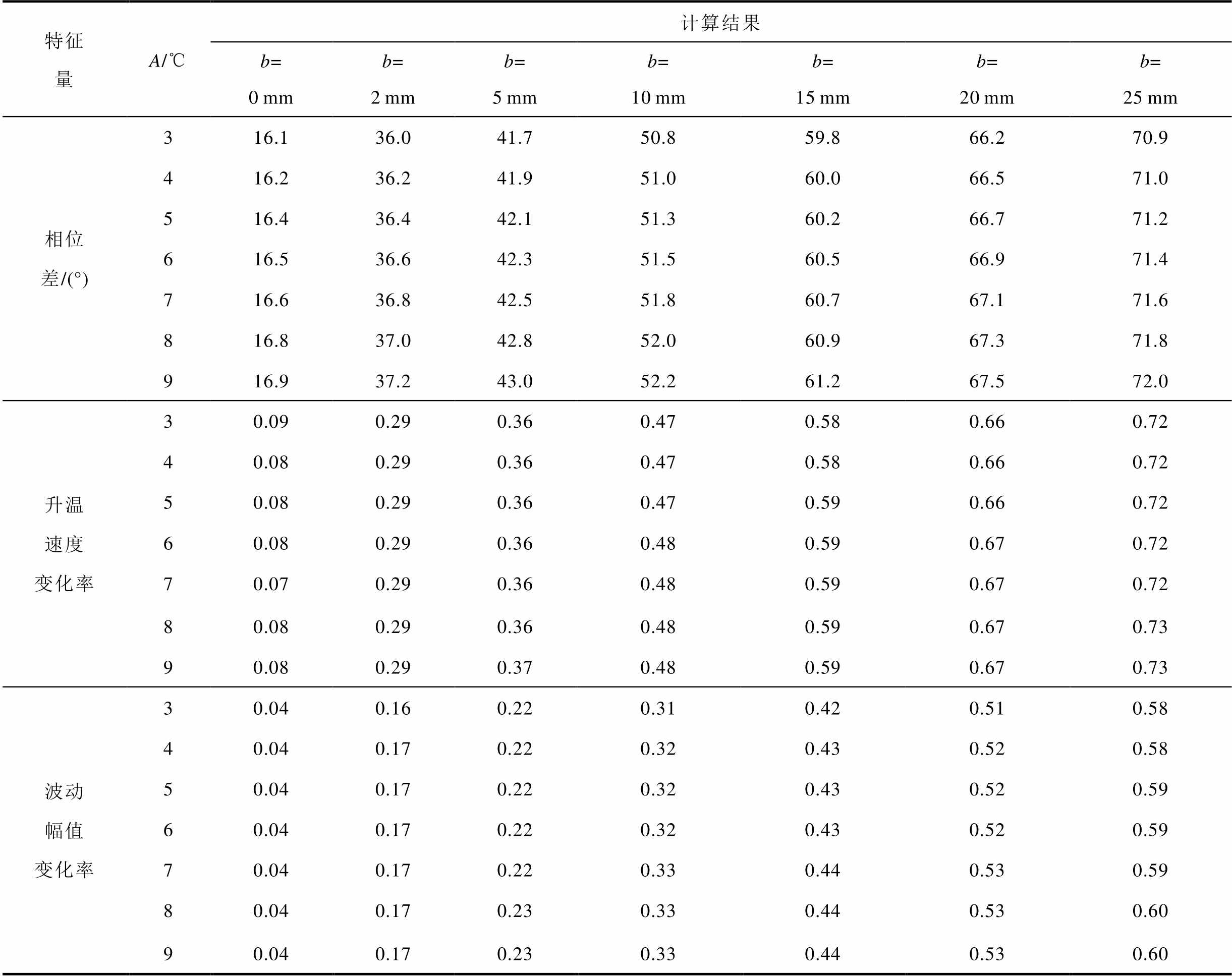
特征量A/℃计算结果 b=0mmb=2mmb=5mmb=10mmb=15mmb=20mmb=25mm 相位差/(°)316.136.041.750.859.866.270.9 416.236.241.951.060.066.571.0 516.436.442.151.360.266.771.2 616.536.642.351.560.566.971.4 716.636.842.551.860.767.171.6 816.837.042.852.060.967.371.8 916.937.243.052.261.267.572.0 升温速度变化率30.090.290.360.470.580.660.72 40.080.290.360.470.580.660.72 50.080.290.360.470.590.660.72 60.080.290.360.480.590.670.72 70.070.290.360.480.590.670.72 80.080.290.360.480.590.670.73 90.080.290.370.480.590.670.73 波动幅值变化率30.040.160.220.310.420.510.58 40.040.170.220.320.430.520.58 50.040.170.220.320.430.520.59 60.040.170.220.320.430.520.59 70.040.170.220.330.440.530.59 80.040.170.230.330.440.530.60 90.040.170.230.330.440.530.60
由表7和表8可知,覆冰厚度对三个特征量的影响较为明显,环境温度均值和波动幅值对相位差、升温速度变化率与波动幅值变化率影响较小。当覆冰厚度分别为0、2、5、10、15、20、25 mm时,式(14)对应的覆冰厚度估算误差最大分别为0.11、0.89、0.44、0.91、1.10、1.30、0.59 mm,式(15)对应的覆冰厚度估算误差最大分别为0.10、0.63、0.29、0.84、0.67、0.96、0.43 mm,式(16)对应的覆冰厚度估算误差最大分别为0.46、1.17、0.34、1.28、0.70、0.94、0.71 mm。因此,在不同环境温度均值和波动幅值的工况下,式(14)~式(16)均能实现覆冰厚度的有效估算。
表8 不同覆冰厚度时的覆冰厚度估算误差
Tab.8 Estimation error in ice thickness at different ice thicknesses
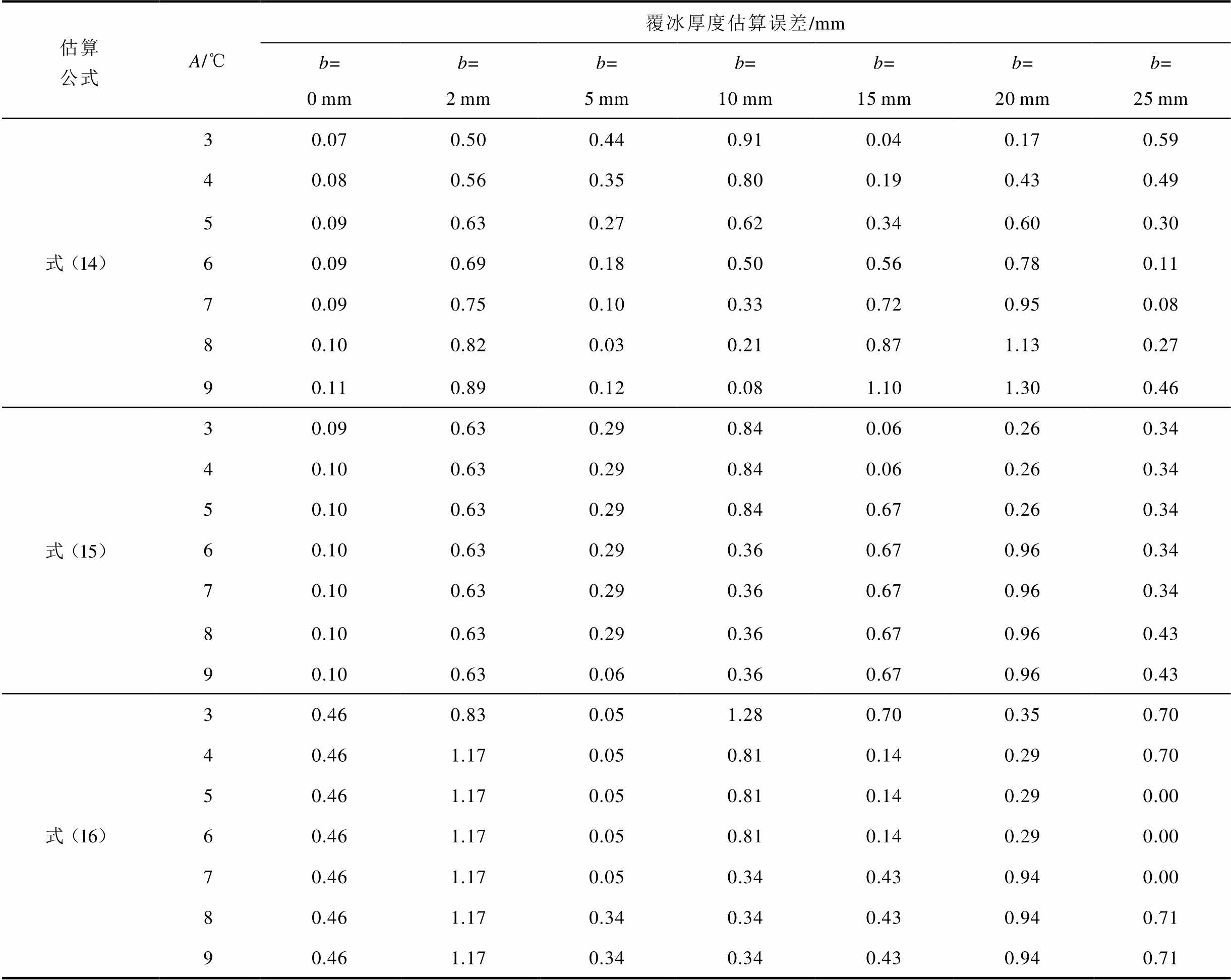
估算公式A/℃覆冰厚度估算误差/mm b=0mmb=2mmb=5mmb=10mmb=15mmb=20mmb=25mm 式(14)30.070.500.440.910.040.170.59 40.080.560.350.800.190.430.49 50.090.630.270.620.340.600.30 60.090.690.180.500.560.780.11 70.090.750.100.330.720.950.08 80.100.820.030.210.871.130.27 90.110.890.120.081.101.300.46 式(15)30.090.630.290.840.060.260.34 40.100.630.290.840.060.260.34 50.100.630.290.840.670.260.34 60.100.630.290.360.670.960.34 70.100.630.290.360.670.960.34 80.100.630.290.360.670.960.43 90.100.630.060.360.670.960.43 式(16)30.460.830.051.280.700.350.70 40.461.170.050.810.140.290.70 50.461.170.050.810.140.290.00 60.461.170.050.810.140.290.00 70.461.170.050.340.430.940.00 80.461.170.340.340.430.940.71 90.461.170.340.340.430.940.71
3.1.4 光纤温度噪声的影响
本小节在覆冰段光纤温度数据存在测量误差时,对上述基于三个特征量的覆冰厚度估算公式进行比较。
环境温度变化采用WAVE法模拟。令B=-A,A=3、5、7℃,b=10 mm,仿真时间为168 h,其余参数均与1.2节中保持一致。考虑实际利用BOTDR对线路温度进行测量时存在的测量误差与连续两次测量之间的时间间隔,设置测量参数如下:每隔0.2 h测量一次光纤温度,并加入均值μT为0℃、标准差σT分别为0.2、0.4、0.6、0.8℃的高斯白噪声模拟BOTDR可能存在的测量误差,每个参数组合下各仿真产生1 000组含噪声的光纤温度数据。以A= 5℃、不同噪声标准差各取一组的数据为例,得到加入噪声时覆冰段光纤温度如图13所示。当时间间隔过小(0.2 h)时,噪声导致升温速度计算误差较大,而时间间隔取1 h时误差整体较小,故时间间隔选择1 h计算三个温度滞后特征量。计算得到三个特征量后分别代入式(14)~式(16),可以得到不同覆冰厚度下的覆冰厚度估算误差。对相同条件下的1 000组含噪光纤温度数据对应的覆冰厚度估算误差取均值,所得结果见表9。
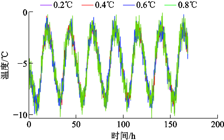
图13 加入噪声时覆冰段光纤温度
Fig.13 Noisy temperature of optical fiber in ice covered section
表9 不同光纤温度噪声下的覆冰厚度估算误差均值
Tab.9 Mean estimation error in ice thickness at different noise levels in measured optical fiber temperature
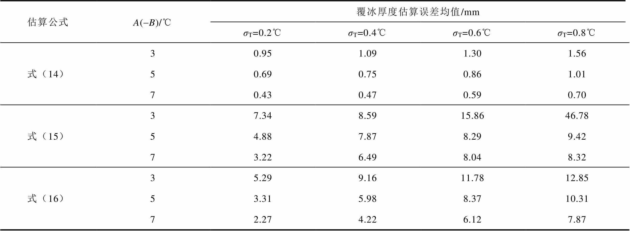
估算公式A(-B)/℃覆冰厚度估算误差均值/mm σT=0.2℃σT=0.4℃σT=0.6℃σT=0.8℃ 式(14)30.951.091.301.56 50.690.750.861.01 70.430.470.590.70 式(15)37.348.5915.8646.78 54.887.878.299.42 73.226.498.048.32 式(16)35.299.1611.7812.85 53.315.988.3710.31 72.274.226.127.87
由表9可知,实际利用BOTDR对线路温度进行测量时,存在的测量误差对基于升温速度变化率与波动幅值变化率的覆冰厚度估算结果影响较为明显。升温速度变化率和波动幅值变化率依赖极值点提取,易受瞬时温度波动干扰,测量误差的存在导致难以准确地得到覆冰段光纤温度曲线在24 h内升温速度的最大值和覆冰段光纤温度曲线在24 h内的峰峰值,使由式(15)和式(16)得到的结果产生了较大误差,对应的覆冰厚度估算误差较大。而测量误差对温度曲线相位差的影响较小,当噪声标准差分别为0.2、0.4、0.6、0.8℃时,对应的覆冰厚度估算误差均值最大分别为0.95、1.09、1.30、1.56 mm,这是因为相位差反映温度曲线的整体周期性滞后特性,通过DFT算法提取基频相位,可有效地抑制局部噪声和测量误差的影响。当存在测量误差与采样间隔较小时,温度曲线相位差最稳定可靠,作为线路覆冰判别特征量更具优势。
基于1.2节中人工气候室内开展的OPGW覆冰温度测量试验获取的光纤温度,对上述覆冰厚度评估公式进行验证。5 mm覆冰时光纤与环境温度随时间的变化如图6所示。
根据图6中的数据结合式(11)~式(13)计算得到的φ、rv和ra分别为39.3°、0.58和0.29。试验环境温度变化下,不同特征量的覆冰厚度估算公式通过与2.2节相同的方法得到,分别为
 (17)
 (18)
 (19)
将得到的特征量分别代入式(17)~式(19),可以得到覆冰厚度为5 mm时,与三个特征量对应的覆冰厚度估计值分别为4.22、12.50、8.08 mm,评估误差分别为0.78、7.50、3.08 mm。当采用温度曲线之间的相位差时,对应的覆冰厚度估算公式具有最小的估算误差。需要注意的是,若温度滞后特征量选择不当,覆冰厚度估算误差最高可扩大8倍。
本文建立了覆冰OPGW的三维温度场模型,通过仿真计算发现了线路温度相对环境温度存在滞后效应,提出了光纤与环境温度曲线间的相位差、升温速度变化率与波动幅值变化率三个温度滞后特征量,并分别给出了对应的覆冰厚度估算公式。进一步分析环境温度均值、波动幅值与光纤温度测量误差对三个估算公式的影响,并开展试验验证,主要结论如下:
1)环境温度均值和波动幅值对光纤与环境温度曲线之间的相位差、升温速度变化率及波动幅值变化率这三个特征量的影响较小,可忽略不计,所提出的公式可有效估算覆冰厚度。
2)光纤温度的测量误差对升温速度变化率与波动幅值变化率的影响较为明显,进而导致覆冰厚度评估误差偏大。经试验与仿真结果验证,温度曲线相位差最稳定可靠,作为输电线路覆冰判别特征量更具优势。若温度滞后特征量选择不当,覆冰厚度估算误差最高可扩大8倍。
参考文献
[1] Rui Xiaoming, Ji Kunpeng, Li Lin, et al. Dynamic response of overhead transmission lines with eccentric ice deposits following shock loads[J]. IEEE Transactions on Power Delivery, 2017, 32(3): 1287-1294.
[2] 牛涛, 黄骞谦, 方斯顿, 等. 基于多光谱卫星遥感的输电网冰灾场景时序建模与韧性提升策略优化[J]. 电工技术学报, 2025, 40(13): 4200-4215, 4305. Niu Tao, Huang Qianqian, Fang Sidun, et al. Temporal modeling of ice disaster scenarios and optimization of resilience enhancement strategies in power transmis-sion network based on multispectral satellite remote sensing data[J]. Transactions of China Electrotechnical Society, 2025, 40(13): 4200-4215, 4305.
[3] Han Shunjie, Li Dongqi, Li Keyu, et al. Analysis and study of transmission line icing based on grey correlation Pearson combinatorial optimization support vector machine[J]. Measurement, 2024, 236: 115086.
[4] 蒋兴良, 孟志高, 张志劲, 等. OPGW临界融冰电流及其影响因素[J]. 电工技术学报, 2016, 31(9): 174-180. Jiang Xingliang, Meng Zhigao, Zhang Zhijin, et al. Critical ice-melting current of ice-covered OPGW and its impacting factors[J]. Transactions of China Electrotechnical Society, 2016, 31(9): 174-180.
[5] 曾伟, 蒋兴良, 杨国林, 等. 基于记忆合金双程形状记忆效应的导线雾凇防冰方法及现场试验[J]. 电工技术学报, 2024, 39(7): 2174-2183. Zeng Wei, Jiang Xingliang, Yang Guolin, et al. Research on anti-icing method for fog freezing and field test of wires based on two-way shape memory effect of memory alloy[J]. Transactions of China Electrotechnical Society, 2024, 39(7): 2174-2183.
[6] 王增平, 曹辰, 王彤. 覆冰区域电网线路停运事故的评估方法[J]. 电工技术学报, 2025, 40(19): 6151-6166. Wang Zengping, Cao Chen, Wang Tong. Assessment method for outages of iced regional power grid lines [J]. Transactions of China Electrotechnical Society, 2025, 40(19): 6151-6166.
[7] Li Ran, Zhang Zhijin, Jiang Xingliang, et al. An online monitoring device for twist angle of iced single conductor of transmission line[J]. IEEE Sensors Journal, 2025, 25(9): 14850-14859.
[8] Qin Zhuoke, Jia Bin, Shen Xiahui, et al. A monitoring method for the ice shape and the freeze-thaw process of ice accretion on transmission line based on circular FBG plane principal strain sensor[J]. IEEE Sensors Journal, 2025, 25(13): 24265-24275.
[9] 范晓舟, 袁洁平, 薛峰, 等. 基于简支绕组横梁算法的变压器绕组形变矢量化监测模型[J]. 电工技术学报, 2025, 40(5): 1639-1651. Fan Xiaozhou, Yuan Jieping, Xue Feng, et al. Vectorization monitoring model of transformer winding deformation based on simply supported winding beam algorithm[J]. Transactions of China Electrotechnical Society, 2025, 40(5): 1639-1651.
[10] Liu Shuaiqi, Yu Feihong, Hong Rui, et al. Advances in phase-sensitive optical time-domain reflectometry [J]. Opto-Electronic Advances, 2022, 5(3): 200078.
[11] 尚秋峰, 王若楠.基于GADF-GCBAM-ResNet的DAS周界安防信号识别方法[J]. 光通信技术, 2026, 50(4): 60-64. Shang Qiufeng, Wang Ruonan. A method for perimeter security signal recognition based on GCBAM-ResNet and DAS[J]. Optical Communication Technology, 2026, 50(4): 60-64.
[12] Guo Haohan, Liu Kun, Li Yuanyao, et al. Single-ended > 100-km distributed vibration sensor based on OFDR using Pearson correlation coefficient[J]. IEEE Sensors Journal, 2025, 25(9): 15143-15154.
[13] Nilakanta Meitei S, Borah K, Chatterjee S. Review on monitoring of transformer insulation oil using optical fiber sensors[J]. Results in Optics, 2023, 10: 100361.
[14] Ding Zhewen, Zhang Xuping, Zou Ningmu, et al. Phi-OTDR based on-line monitoring of overhead power transmission line[J]. Journal of Lightwave Technology, 2021, 39(15): 5163-5169.
[15] Buchmayer F, Monsberger C M, Lienhart W. Advantages of tunnel monitoring using distributed fibre optic sensing[J]. Journal of Applied Geodesy, 2021, 15(1): 1-12.
[16] 郝艳捧, 毛典明, 成延庭, 等. BOTDR监测OPGW覆冰最小临界厚度试验方法[J]. 高电压技术, 2025, 51(7): 3191-3200. Hao Yanpeng, Mao Dianming, Cheng Yanting, et al. Test method for minimum critical thickness of ice coating on OPGW based on BOTDR monitoring[J]. High Voltage Engineering, 2025, 51(7): 3191-3200.
[17] 董乃臻,肖海, 刘云鹏, 等. 基于分布式动态应变传感的光纤复合相线脱冰跳跃监测技术[J]. 电工技术学报, 2026, 41(7): 2484-2497. Dong Naizhen, Xiao Hai, Liu Yunpeng, et al. De-icing jump monitoring technology of optical fiber composite phase conductor based on distributed dynamic strain sensing[J]. Transactions of China Electrotechnical Society, 2026, 41(7): 2484-2497.
[18] 张旭苹, 张益昕, 王亮, 等. 分布式光纤传感技术研究和应用的现状及未来[J]. 光学学报, 2024, 44(1): 0106001. Zhang Xuping, Zhang Yixin, Wang Liang, et al. Current status and future of research and applications for distributed fiber optic sensing technology[J]. Acta Optica Sinica, 2024, 44(1): 0106001.
[19] 吴春芳, 陈云, 黄韬, 等. 电力电缆状态感知与检测技术研究综述[J]. 高压电器, 2024, 60(10): 86-103. Wu Chunfang, Chen Yun, Huang Tao, et al. Overview of condition sensing and detection technology for power cables[J]. High Voltage Apparatus, 2024, 60(10): 86-103.
[20] 吴念, 王海涛, 张宗峰, 等. 基于OPGW的输电线路覆冰广域监测方法[J]. 中国电力, 2017, 50(5): 65-70. Wu Nian, Wang Haitao, Zhang Zongfeng, et al. Research of transmission line icing wide-area monitoringbased on OPGW[J]. Electric Power, 2017, 50(5): 65-70.
[21] 覃兆宇, 刘卫新, 潘哲哲, 等. 光纤布里渊分布式输电线路覆冰识别技术[J]. 光电工程, 2016, 43(10): 6-11. Qin Zhaoyu, Liu Weixin, Pan Zhezhe, et al. Optical Brillouin distributed ice-coating identification technology on transmission line[J]. Opto-Electronic Engineering, 2016, 43(10): 6-11.
[22] Sun Jinxiang, Zhang Zhiguo, Li Yuemei, et al. Distributed transmission line ice-coating recognition system based on BOTDR temperature monitoring[J]. Journal of Lightwave Technology, 2021, 39(12): 3967-3973.
[23] Zou Xiaoming, Liu Xinzhan, He Yi, et al. Ice thickness estimation method of overhead line based on distributed optical fiber temperature sensing[C]// Proceedings of the Sixth International Conference on Energy Engineering and Environmental Protection, Sanya, China, 2021: 012071.
[24] 徐志钮, 李先锋, 郭一帆, 等. 基于温度滞后相位的输电线路覆冰监测方法[J]. 电力工程技术, 2022, 41(6): 91-100. Xu Zhiniu, Li Xianfeng, Guo Yifan, et al. Icing monitoring method of transmission lines based on temperature lagging phase[J]. Electric Power Engineering Technology, 2022, 41(6): 91-100.
[25] Luo Jianbin, Hao Yanpeng, Ye Qing, et al. Development of optical fiber sensors based on Brillouin scattering and FBG for on-line monitoring in overhead transmission lines[J]. Journal of Lightwave Technology, 2013, 31(10): 1559-1565.
[26] 范鹏, 刘春翔, 姜德华, 等. OPGW受拉力时光纤的应变分析[J]. 电线电缆, 2015, 58(4): 10-13, 25. Fan Peng, Liu Chunxiang, Jiang Dehua, et al. Stress and strain analysis of the optical fibers in an OPGW[J]. Electric Wire & Cable, 2015, 58(4): 10-13, 25.
[27] Zunec M, Ticar I, Jakl F. Determination of current and temperature distribution in overhead conductors by using electromagnetic-field analysis tools[J]. IEEE Transactions on Power Delivery, 2006, 21(3): 1524-1529.
[28] Ashfaq A, Khalique U, Nadeem A, et al. Comprehensive analysis of temperature distribution in OPGW cable considering ramifications of short circuit current[J]. Scientific Reports, 2025, 15: 21949.
[29] Reicosky D C, Winkelman L J, Baker J M, et al. Accuracy of hourly air temperatures calculated from daily minima and maxima[J]. Agricultural and Forest Meteorology, 1989, 46(3): 193-209.
Abstract Transmission line icing accident is one of the main threats to the normal operation of power system, and its effective monitoring and prevention has become an important issue to ensure the safety of power grid. Distributed optical fiber sensing technology has the advantages of long monitoring distance, high measurement accuracy, and strong resistance to electromagnetic interference. The monitoring of transmission line icing based on this technology is a current research hotspot. However, there are still the following key problems: (1) Most of the research results lack experimental validation. (2) There is no research on the comparison and selection of the temperature lag parameters of icing monitoring. (3) There is also little research on the influence of some key factors on the effectiveness of icing monitoring in practical applications. In this work, based on the experiment and temperature field model of iced transmission line, the monitoring method of transmission line icing based on the lag parameters of temperature is investigated.
In this work, the WAVE method is used to simulate the variation of real environmental temperature with time, a three-dimensional temperature field model for optical fiber composite overhead ground wire (OPGW) during icing is established, and the icing experiments in an artificial climate chamber based on the Brillouin optical time domain reflectometer (BOTDR) is conducted. These experiments validate the model, and meanwhile, the lag characteristic of line temperature is validated through both simulations and experiments. In fact, the temperature lag characteristic is measured according to the Brillouin frequency shift. The Brillouin frequency shift is linear to the temperature and strain of the optical fiber. According to the practical situation of transmission line, the optical fiber strain caused by the iceis essentially constant astime increases. Therefore, the influence of the optical fiber strain on the temperature lag characteristic can be neglected. The temperature lag characteristic of the optical fiber is solely related to the optical fiber temperature. On this basis, three temperature lag parameters are proposed: the phase difference between the optical fiber and environmental temperature curves, the change rate of heating rate, and the change rate of fluctuation amplitude. Through modeling research based on the validated temperature field model, the values of the three parameters at different icing thicknesses are obtained, and the corresponding icing thickness estimation formulas are respectively obtained via fitting. The model is used to analyze the effects of environmental temperature variation and optical fiber temperature measurement error on the three parameters. Furthermore, through the optical fiber temperature measurement based on BOTDR, noisy optical fiber temperature data are acquired. Based on this data, the impact of the temperature measurement error on the calculation accuracy of the above three formulas is investigated and a compared.
The conclusions are as follows: (1) The mean value and fluctuation amplitude of environmental temperature have relatively small effects on the phase difference, the variation in maximum change of rate and amplitude between the optical fiber and the ambient temperature curves, which can be ignored and the proposed formulas of three parameters can be used to estimate the ice thickness. (2) The optical fiber temperature measurement error has a significant influence on the change rate of heating rate and the change rate of fluctuation amplitude, but has a minor impact on the phase difference. The icing estimation based on the phase difference of temperature curves achieves the highest accuracy. And if the temperature lag parameters are improperly selected, the error in icing thickness estimation can differ by up to 8 times.
keywords:Optical fiber composite overhead ground wire (OPGW), Brillouin optical time domain reflectometry (BOTDR), icing criterion, temperature hysteresis parameter, monitoring of ice thickness
DOI: 10.19595/j.cnki.1000-6753.tces.251767
中图分类号:TM75
国家自然科学基金资助项目(62171185, 62273146)。
收稿日期 2025-10-15
改稿日期 2025-12-22
徐志钮 男,1979年生,博士,教授,博士生导师,研究方向为光纤分布式传感及其在电气设备状态监测与故障诊断中的应用。E-mail:wzcnjxx@163.com
赵丽娟 女,1981年生,博士,教授,博士生导师,研究方向为光纤通信与传感。E-mail:hdzlj@126.com(通信作者)