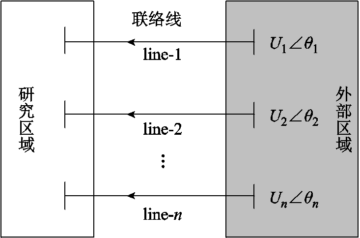
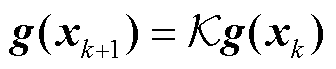
图1 等值区域示意图
Fig.1 Schematic diagram of equivalent areas
摘要 目前尚缺乏能够同时适用于大扰动和小扰动工况的电力系统动态等值建模方法。为提升等值建模方法对电力系统不确定性和时变运行工况的适应能力,该文基于数据驱动方式提出一种电力系统Koopman动态等值方法。首先建立外部系统状态方程和输出方程,通过Koopman算子对其进行高维线性化映射,在高维空间实现外部系统状态空间模型的全局线性化;其次分别通过动态模式分解和最小二乘辨识等值模型状态系数矩阵和输出系数矩阵,并在噪声影响下对模型参数进行修正;然后对状态系数矩阵进行谱分解提取Koopman模态,通过压缩模态数目实现系统降阶;最后设置算例,验证所提方法的合理性。结果表明,在算例系统处于不同程度的扰动下,所提等值模型与原系统具有基本一致的功角摇摆曲线和功率输出曲线,等值模型的准确度为97.74%,并与常用的同调方法和模态方法进行对比,说明了所提方法的鲁棒性和普适性。
关键词:动态等值 Koopman 模态方法 同调方法 不同扰动
随着现代电力系统的发展,各区域电网间的联系越来越密切[1-2]。对大规模电力系统进行仿真分析是电网公司和相关科研、设计单位指导实际电网规划、运行和工程建设的重要工作[3-4]。但电力系统的复杂结构和庞大模型阶数,使其在电磁暂态仿真及动态特性分析中尤为困难。因此在研究大规模区域互联电网时,需要更合适的动态等值模型来替补外部系统[5]。
目前常用的动态等值方法主要为同调方法和模态方法[6-7]。同调方法将具有相近摇摆曲线的发电机分为一组进行网络化简,分别等值成一台或几台等值机[8-9]。文献[10]提出了一种基于Prony分析特征提取的同调机组分群方法,通过提取功角曲线特征识别同调机组;文献[11]考虑了电动机负荷动态特性对发电机的影响,实现了发电机重新分群。同调等值法理论基础充分,但等值发电机及其控制系统等元件参数聚合极为复杂,对于大规模电力系统等值工作量巨大[12-14]。同时,在小扰动下,系统动态特性变化并不明显,不容易辨别同调发电机群,因此同调方法只适用于大扰动下的电力系统等值。
模态方法根据系统各结构动态微分方程建立状态空间矩阵,通过压缩模态数目降低模型阶数[15]。文献[16]通过建立双馈风电机组的状态空间模型分析了其主导特征值对系统状态的影响,并基于特征值实现了系统降阶;文献[17]通过分析风电并网系统的特征值建立了其降阶模型,解释了系统次同步振荡机理。模态方法基于电力系统运行平衡点对非线性系统进行近似线性化。在大扰动下,如短路故障或大型负荷突变,电力系统的动态行为会变得高度非线性,不能满足系统运行平衡点进行线性化的条件,因此模态方法只适用于小扰动下的电力系统动态等值[18-20]。
另外,同调方法和模态方法均需要明确系统详细结构和运行参数。随着电力市场改革的稳步推进,各区域电网为增强所辖电网数据的安全性,提升了信息保密级别,使各区域互联子系统结构信息与实时数据交换尤为困难,极大地限制了同调方法和模态方法的应用[21]。
综上所述,目前常用的等值方法不能适用于不同程度扰动下的电力系统动态等值。此外,随着电力系统规模的扩大和复杂性的增加,建模难度和工作量也在不断增加,传统的等值方法可能无法满足应对电力系统时变性的要求。
据此,本文提出了一种能够适用于不同程度扰动的电力系统Koopman动态等值模型,对不同运行工况下的电力系统动态等值方法进行了统一,以增强等值模型对电力系统不确定性和时变运行工况的适应能力,提高等值模型的鲁棒性和普适性。首先,通过Koopman算子对外部系统状态空间模型进行高维线性化映射,建立外部系统全局线性化模型;其次,分别通过动态模式分解和最小二乘辨识等值模型状态系数矩阵和输出系数矩阵,对系统状态矩阵的谱分解提取Koopman模态,通过压缩模态数据实现系统降阶;最后,设置不同程度扰动算例,验证所提方法的合理性。
在对大型互联电网进行分析过程中,一般只对其中某个局部进行详细研究。电力系统动态等值是保持待研究区域(内部系统)不变,而在保证外部区域(外部系统)与研究区域动态交互过程相等或相近的前提下对外部系统进行简化的过程。等值区域示意图如图1所示。假设在外部区域有n个边界节点,其通过联络线与研究区域进行动态交互。联络线编号为line-1~line-n。
图1 等值区域示意图
Fig.1 Schematic diagram of equivalent areas
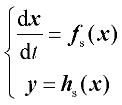
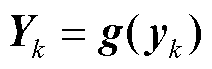
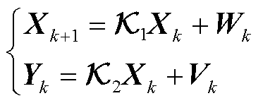
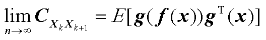
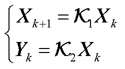
由于研究目标是外部系统自然动态特性和稳定性,因此电力系统外部区域动态模型可由一组状态方程和输出方程描述为
 (1)
(1)
式中,x为系统状态变量;y为系统输出变量; 为系统状态特性函数;
 为系统输出特性函数。
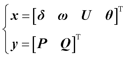
由于外部系统联络线传输功率与发电机状态和边界节点电压水平相关,因此外部系统模型状态变量和输出变量可选择为
 (2)
(2)
式中, 为外部系统发电机功角;ω为外部系统发电机转速;
 和
和 分别为边界节点电压和相角;P和Q分别为外部区域经联络线输出至研究区域系统的有功功率和无功功率。
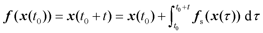
在电力系统中,数据测量采集和处理常采用离散形式,由离散映射关系f将式(1)映射为
 (3)
(3)
式中,f为信号离散时序映射关系;t0为初始时间;τ为中间积分变量;t为系统演化时间,t=k∆t,k为自然数,∆t为离散时间步长。式(1)连续系统离散化后的解集可表示为
 (4)
(4)
式中, ,
, ,
, 。
。
定义Koopman算子 ,其作用在系统观测函数,对系统原信号空间进行高维线性化映射。
 (5)
(5)
式中, ,G为高维Koopman空间,
 为复数域,
为复数域, 。
。
在算子作用下,实现系统由低维非线性空间M到高维Koopman线性空间G的映射,即在Koopman空间中,系统可以实现式(1)系统状态方程线性迭代求解,详细证明过程见附录第1节。
 (6)
(6)
与基于平衡点的模型线性化不同,即使系统状态底层动态是非线性的,但Koopman算子在时间间隔 上的映射是线性的,因此算子并不会随时间而变化。经算子映射,将无法直接求解的非线性状态微分方程转换为式(6)所示Koopman空间中线性迭代方程,实现对系统的全局线性化分析,该过程示意图如图2所示。
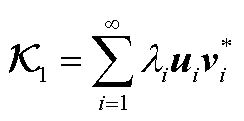
谱分析是求解线性系统常用理论。在高维空间中,对算子进行谱分解为
 (7)
(7)
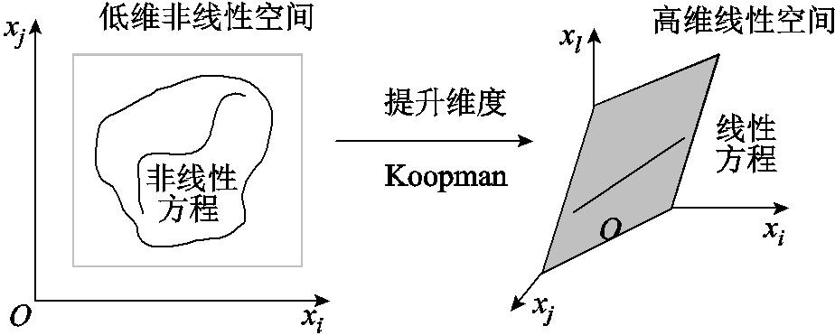
图2 系统升维线性化过程
Fig.2 The process of dimensionality-increasing linearization
式中, 为系统Koopman特征函数;
 为系统特征值。
将观测函数 限制在由Koopman算子特征函数张成的不变子空间中,空间基函数为
 ,观测函数
,观测函数 可表示为
可表示为
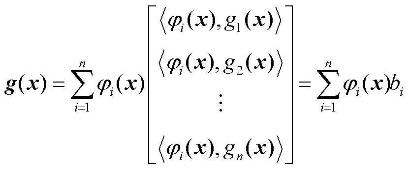 (8)
(8)
式中, 为系统演化系数,计算方法见附录第5节。
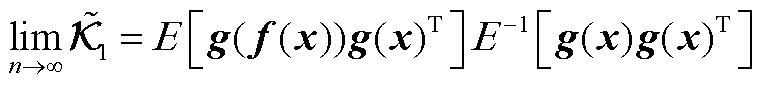
系统任意时刻的解可由Koopman特征值、特征向量和模态线性表示为
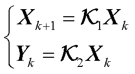
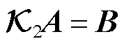
据此,基于式(6)以线性算子描述原系统动态特性,实现等值模型全局线性化。因此外部系统Koopman动态等值模型可表示为
 (10)
(10)
式中,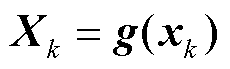 ,
, ;
; 为系统状态系数矩阵;
 为系统输出系数矩阵。模型收敛性由附录第3节推导证明。
第一个方程为系统状态方程,描述了等值区域系统内部状态变量的变化关系。通过状态系数矩阵预测系统未来时刻的状态。第二个方程为系统输出方程,描述了等值区域系统外部输出变量与内部状态的关系。通过输出系数矩阵观测系统输出。
由于外部系统联络线功率传输情况与发电机状态和边界节点电压水平相关,因此可选择外部系统模型状态变量X为外部系统中发电机功角和转速 ,边界节点电压和相角;输出变量Y为外部区域经联络线输出至研究区域系统的有功功率P和无功功率Q。
现代电力系统配备了先进的自动化监测设备,能够实时采集电力系统的各种数据。这些自动化设备能够在极短的时间内完成数据采集任务,确保了数据的实时性。本文所提方法所需数据为等值边界数据和发电机监测数据,均可以通过同步相量测量单元(Phasor Measurement Unit, PMU)等设备实时监测和采集,如广域测量系统(Wide Area Measurement System, WAMS)配套PMU采集速率为2 400点/s,国家电网公司标准PMU、西门子SIPROTEC 5系列PMU采集速率可达4 800点/s,动态数据上传速率为10~50次/s,保障了数据采集方式的实时性和高效性。
下面通过外部系统边界测量数据矩阵 和
和 辨识Koopman等值模型系数矩阵
 和
和 。
。
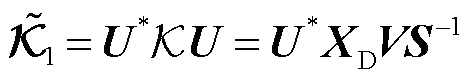
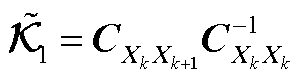
高维Koopman算子在计算中难以应用。本节基于动态模式分解(Dynamic Mode Decomposition, DMD)辨识外部系统状态系数矩阵 ,基于最小二乘辨识外部系统输出系数矩阵
 。
。
 辨识
辨识附录第2节证明了基于DMD对外部系统状态系数矩阵 的低维空间辨识矩阵
 和具有相同的状态空间特性。因此可以通过的谱分解代替求解原模型的数值解。
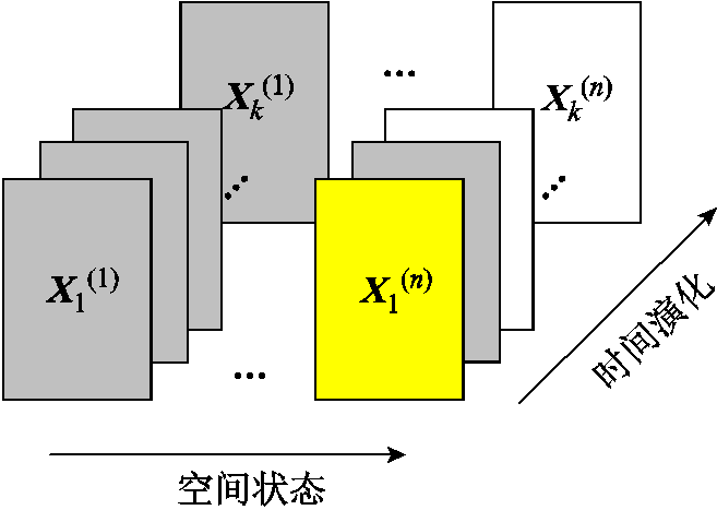
图3 DMD输入数据集时序快照序列
Fig.3 Time series snapshot of input datasets for DMD
基于外部系统状态测量数据X构建外部系统状态数据矩阵XF及其时延矩阵XD为
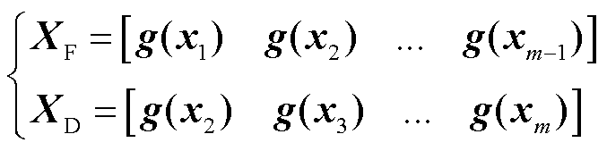 (11)
(11)
对Xk的奇异值分解为
 (12)
(12)
式中,U为系统空间模态, ;V为系统时间模态,
 ,满足
,满足 ,
, ,m为测点数量;S为奇异值对角阵,
 ,r为截断值。
 可以表示为
可以表示为
 (13)
(13)
算子的辨识值为最小Frobenius范数解,有
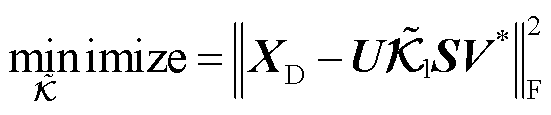 (14)
(14)
式中,minimize为求解函数最小值。
求解式(14)可得 的低维辨识值为
 (15)
(15)
 谱分解的连续特征值
 和离散特征值转换关系为
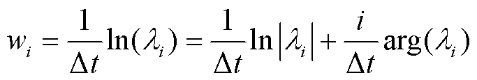 (16)
(16)
式中,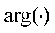 为求辐角。
为求辐角。
对于第i个特征值,如果wi处于虚轴左侧,则该模态将会随时间衰减,且离虚轴越远则衰减越快。wi的虚部决定该模态的振荡频率,离实轴越远,振荡频率越高;反之,振荡频率越低。特征值越靠近虚轴的模态对系统影响越大,将会主导系统动态特性。而快速衰减的模态对系统动态特性影响相对较小。保留对系统影响较大的模态进行分析,滤除快速衰减模态,可以实现系统降阶,显著减少计算量。
 辨识
辨识通过最小化观测点与输出方程差值辨识输出系数矩阵 最优解,建立目标函数为
式中,N为测点数; 为测量输出数据矩阵。式(17)可展开为
![]() (18)
(18)
式中,tr(·)表示矩阵的迹。
令式(18)对 的导数
的导数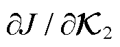 为0,可得
为0,可得
式(19)整理为
 (20)
(20)
解得式(17)最优 辨识值为
辨识值为
 (21)
(21)
式中,![]() ;
;![]() 。
。
据此,Koopman等值模型状态系数矩阵 和输出系数矩阵
 可由式(15)和式(21)辨识得到。
本节考虑在测量信号含有噪声时,模型修正为
 (22)
(22)
式中,Wk和Vk为互不相关的白噪声序列,其统计特性为
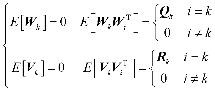 (23)
(23)
式中,E为期望, 。
。
通过总体最小二乘动态模式分解(Total Least Squares-Dynamic Mode Decomposition, TLS-DMD)分离信号空间中的真实模态与噪声模态。对增广数据矩阵D1的奇异值分解(Singular Value Decomposition, SVD)为
 (24)
(24)
其中
噪声模态频率高,能量占比小。D. L. Donoho 和S. T. M. Dawson 等证明了可以通过中值奇异值 计算滤除观测数据矩阵噪声的最优截断阈值ε[22-23],保留大于噪声阈值的奇异值,而滤除低于噪声阈值的奇异值。最优噪声截断阈值τ为
 (25)
(25)
式中, ,
, 为Marcenko-Pastur分布的中位数,
 ,
, 为
为
 (26)
(26)
滤除噪声模态后,状态系数矩阵可辨识为
 (27)
(27)
式中, 为Moore-Penrose逆。
TLS通过最小化观测点到输出方程曲线垂直距离平方和辨识噪声影响下输出系数矩阵最优解,建立目标函数为
 (28)
(28)
构造增广数据协方差矩阵为
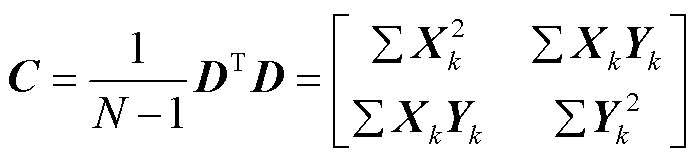 (29)
(29)
式中,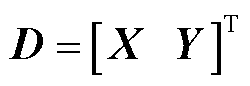 。
。
通过协方差矩阵最小特征值对应的特征向量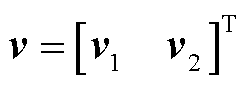 ,可求得式(28)的TLS解,即在噪声影响下
 可辨识为
可辨识为
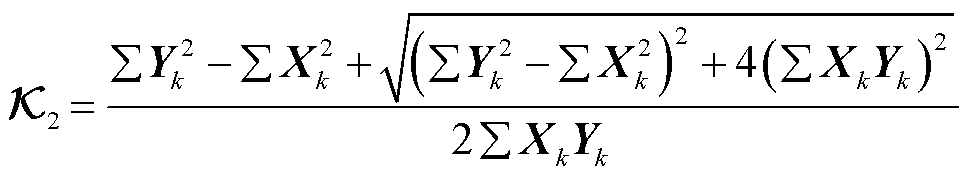 (30)
(30)
引入决定系数(Coefficient of Determination, R²)作为本文模型预测精度评价指标,其定义为
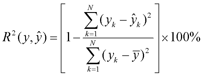 (31)
(31)
式中,N为测点数; 和
和 分别为第k个序列样本的真值和预测值;
 为所有时序样本平均值。
该评价模型不受观察尺度的影响,R2越接近1,代表模型预测精度越高。定义方均根误差(Root Mean Squared Error, RMSE)和平均绝对误差(Mean Absolute Error, MAE)作为评价误差大小指标,RMSE和MAE的值越小,代表模型误差越小。
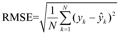 (32)
(32)
![]() (33)
(33)
依据实际工程要求,曲线拟合精度R2达到90%以上可以满足误差要求,即等值模型可以代替原系统进行动态特性分析。
本节设计算例,基于PSASP搭建39节点电力系统,并在不同扰动程度下对所提方法进行测试,验证所提方法对电力系统不同运行工况下的适用效果。
39节点电力系统单线图如图4所示,系统包含10台发电机、39个母线节点、交直流线路以及换流站和控制设备等。对系统阴影区域包括4台发电机13个节点的外部系统进行动态等值。
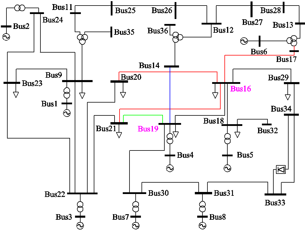
图4 39节点电力系统单线图
Fig.4 Single-Line Diagram of the 39-Bus System
外部系统边界节点为Bus16和Bus19,外部系统边界节点与研究系统边界节点间联络线分别为Line19-14、Line19-21、Line16-17、Line16-20和Line16-21。外部系统经联络线传输至研究系统的功率为系统输出,外部系统内发电机功角、转速和边界节点电压状态为系统状态。
系统在0 s时已进入稳态。对系统分别施加以下两种不同程度的扰动,验证所提方法在算例系统不同运行工况下的等值效果。
(1)大扰动设置:对节点26设置三相接地故障,持续时间为0.1 s。
(2)小扰动设置:对9节点设置随机负荷扰动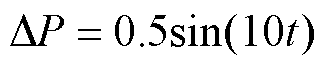 。
。
测量并采集外部系统边界电气量信号,组成9 000个时序序列样本,构建实测动态数据集和,信号采集时间间隔∆t为0.001 s,辨识Koopman等值模型状态系数矩阵 和输出系数矩阵
 。
。
 辨识
辨识在系统大扰动运行状态下,依据式(7)提取的系统Koopman特征值及模态特性结果见表1。
外部系统连续特征值分布如图5所示。由图5可以看出,集中在虚轴附近的虚线框内黄色模态衰减很慢,这些模态是对外部系统影响较大的模态,主导了系统的动态特性。蓝色模态距离离虚轴较远,随时间增长会迅速衰减,对系统动态特性影响较小,这些模态的动态特性主要由系统中受扰动源影响很小的节点区域状态组成。因此,可以保留受扰动源影响较大的Koopman模态(黄色模态),而滤除对系统影响较小的模态(蓝色模态),对外部系统Koopman等值模型进行进一步降阶。
表1 外部系统测量数据特征值提取结果
Tab. 1 Extraction results of characteristic value from external system measurement data
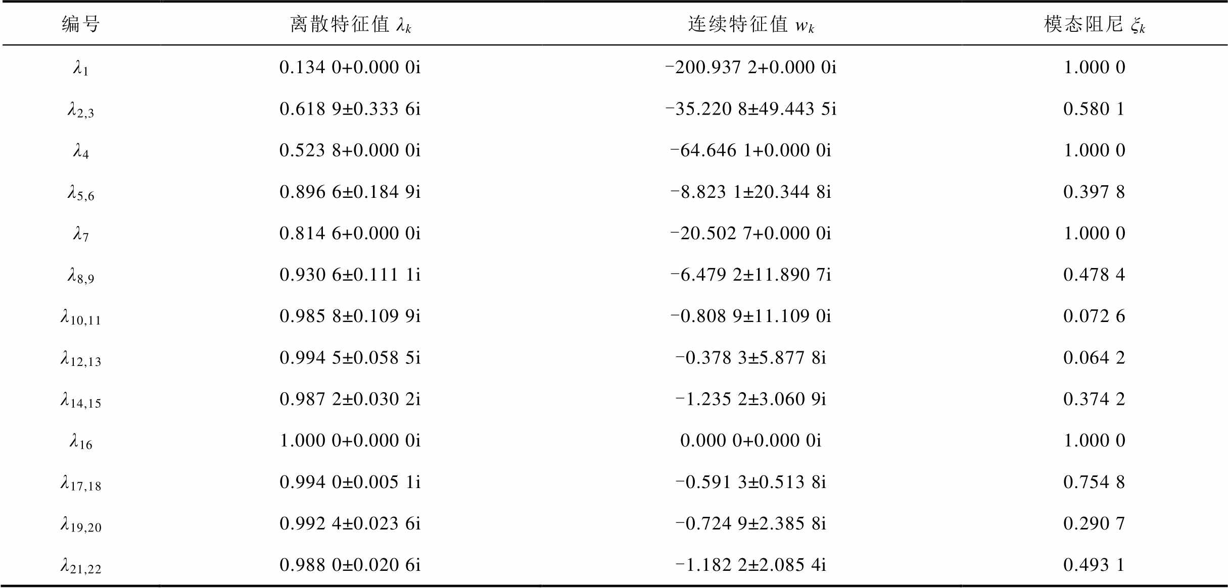
编号离散特征值λk连续特征值wk模态阻尼ξk λ10.134 0+0.000 0i-200.937 2+0.000 0i1.000 0 λ2,30.618 9±0.333 6i-35.220 8±49.443 5i0.580 1 λ40.523 8+0.000 0i-64.646 1+0.000 0i1.000 0 λ5,60.896 6±0.184 9i-8.823 1±20.344 8i0.397 8 λ70.814 6+0.000 0i-20.502 7+0.000 0i1.000 0 λ8,90.930 6±0.111 1i-6.479 2±11.890 7i0.478 4 λ10,110.985 8±0.109 9i-0.808 9±11.109 0i0.072 6 λ12,130.994 5±0.058 5i-0.378 3±5.877 8i0.064 2 λ14,150.987 2±0.030 2i-1.235 2±3.060 9i0.374 2 λ161.000 0+0.000 0i0.000 0+0.000 0i1.000 0 λ17,180.994 0±0.005 1i-0.591 3±0.513 8i0.754 8 λ19,200.992 4±0.023 6i-0.724 9±2.385 8i0.290 7 λ21,220.988 0±0.020 6i-1.182 2±2.085 4i0.493 1
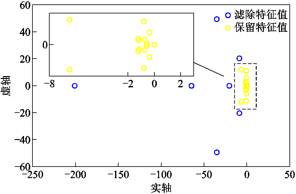
图5 外部系统连续特征值分布
Fig.5 Distribution of characteristic values of external systems
对系统状态的等值结果如图6所示。可以看出,在故障下,外部系统原模型与等值模型功角摇摆曲线基本吻合。说明在大扰动下,等值系统和原系统具有一致的动态稳定性。
图7对比了在发生故障下,原系统和Koopman等值模型边界节点电压变化。可以看出,在发生故障后,系统电压突然发生跌落,等值模型可以较好地还原系统电压的最小值,并在故障切除后,具有和原系统几乎一致的电压恢复特性曲线。
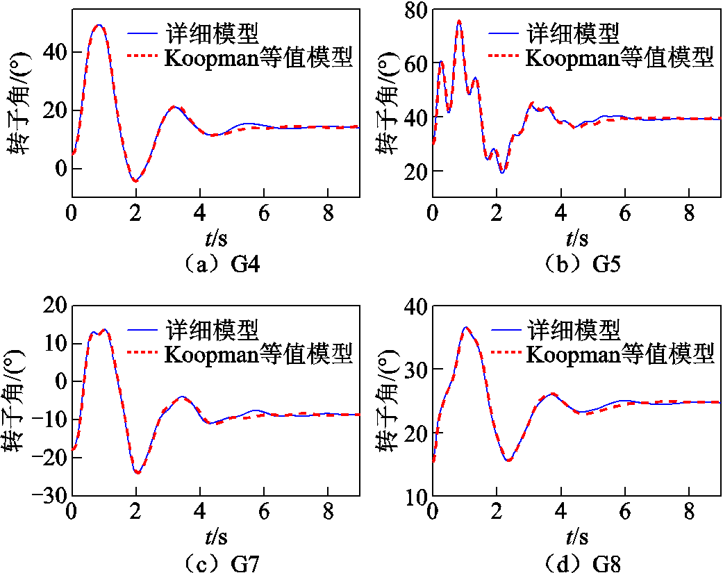
图6 等值前后外部系统发电机功角摇摆曲线对比
Fig.6 Comparison of power angle swing curves of external system generators before and after equivalence
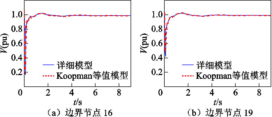
图7 等值前后边界节点电压恢复曲线对比
Fig.7 Comparison of boundary node voltages before and after equivalencing
 辨识
辨识所提模型与原系统对边界联络线Line19-14、Line19-21、Line16-17、Line16-20和Line16-21的功率响应曲线如图8~图12所示。
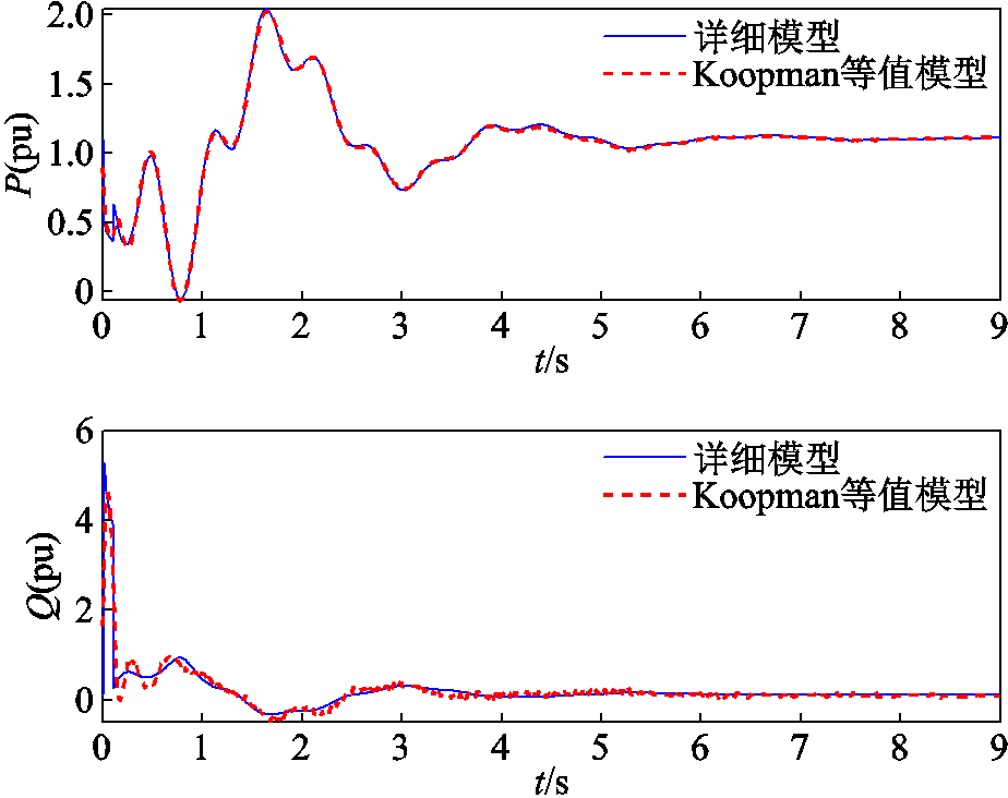
图8 联络线Line19-14传输功率对比
Fig.8 Comparison of transmission power on interconnection line 19-14
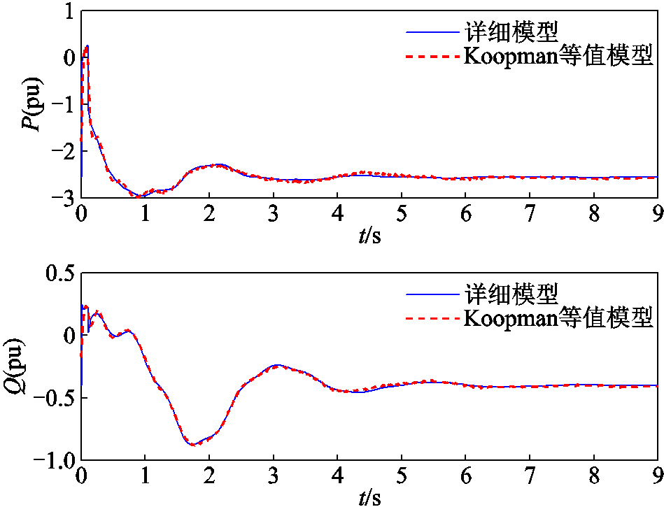
图9 联络线Line19-21传输功率对比
Fig.9 Comparison of transmission power on interconnection line 19-21
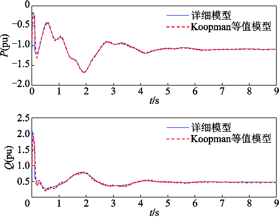
图10 联络线Line16-17传输功率对比
Fig.10 Comparison of transmission power on interconnection line 16-17
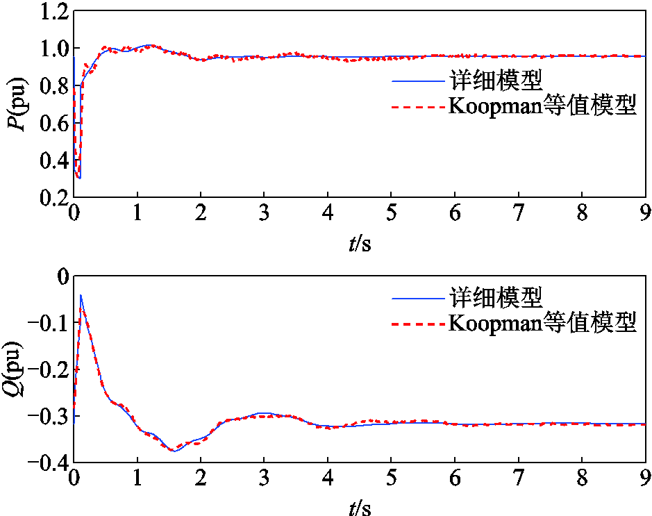
图11 联络线Line16-20传输功率对比
Fig.11 Comparison of transmission power on interconnection line 16-20
由图8~图12可以看出,等值模型和原模型联络线传输有功功率P和无功功率Q基本一致。在故障发生后,系统电压迅速跌落。系统无功补偿装置迅速动作发出无功功率,对系统电压水平起支撑和恢复作用,等值系统和原系统具有基本一致的无功补偿曲线。说明等值模型较好地捕捉了原外部系统的动态特性,具有较好的等值效果,可以替补原系统在大扰动下进行暂态稳定分析。
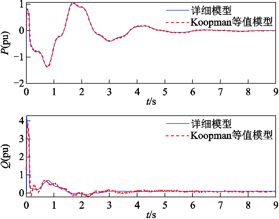
图12 联络线Line16-21传输功率对比
Fig.12 Comparison of transmission power on interconnection line 16-21
大扰动下系统Koopman动态等值模型见附表1、附表2。
本节给出了算例系统在小扰动下的外部系统动态等值结果,验证所提方法等值效果。小扰动下系统Koopman动态等值模型见附表3、附表4。
等值前后外部系统发电机功角摇摆曲线对比如图13所示。可以看出,在小扰动干扰下,系统动态特性变化并不明显,发电机功角呈现小范围波动。等值模型与原系统具有基本一致的功角摇摆曲线,说明等值模型和原系统具有一致的动态稳定性。
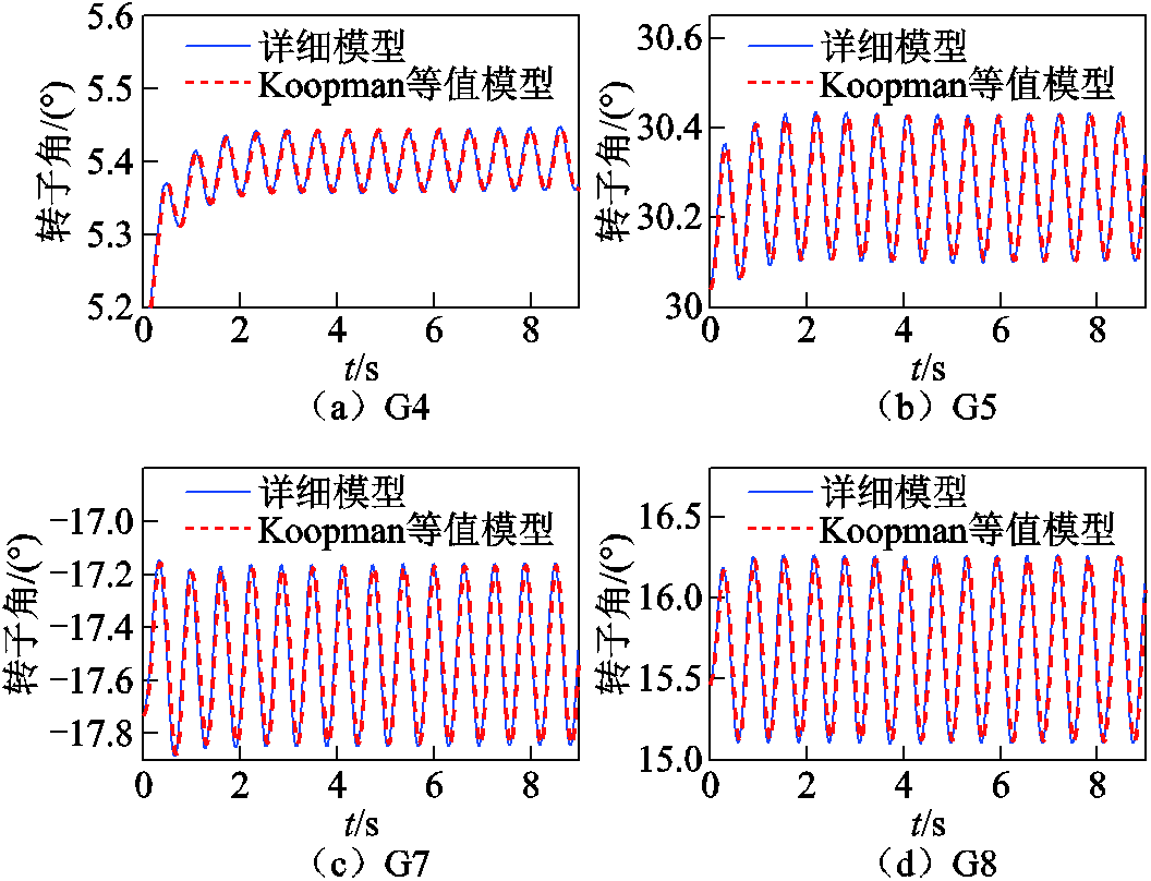
图13 等值前后外部系统发电机功角摇摆曲线对比
Fig.13 Comparison of power angle swing curves of external system generators before and after equivalence
等值前后外部系统联络线传输功率对比如图14所示。图14给出了小扰动下所提模型和原模型对外部系统与研究系统边界联络线Line19-14、Line19-21、Line16-17、Line16-20和Line16-21的功率响应曲线。可以看出,等值模型与原模型联络线输送功率基本一致,说明可以使用所提等值模型替补原系统在小扰动下进行静态稳定分析。
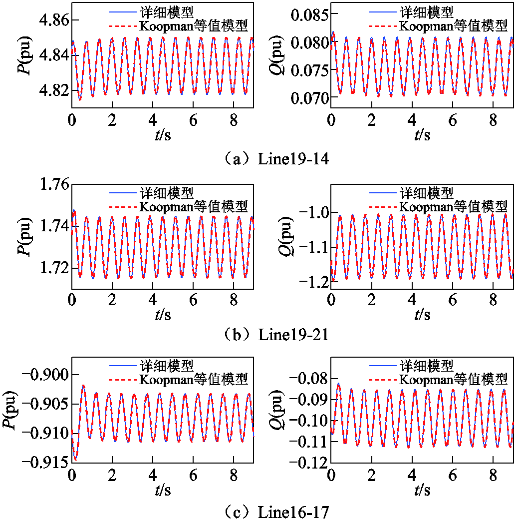
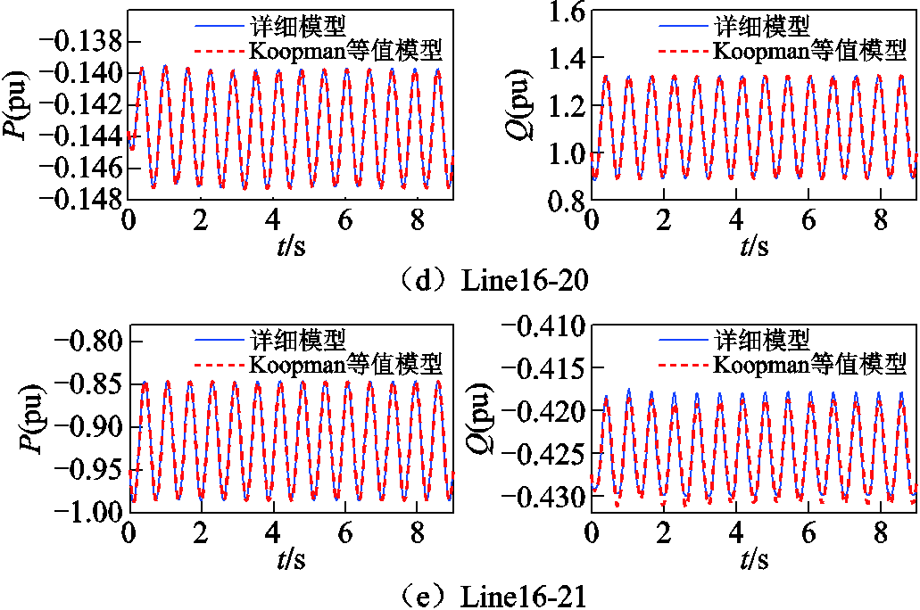
图14 等值前后外部系统联络线传输功率对比
Fig.14 Comparison of transmission power on external system interconnection lines before and after equivalence
本节以大扰动下所提方法对外部系统等值结果为例,定量评估所提模型的等值效果。依据式(31)~式(33)所提指标计算网络等值前后边界潮流误差和等值模型精度,结果见表2。
表2 外部系统等值前后边界联络线传输功率误差和等值模型精度
Tab. 2 The error in boundary tie lines transmission power before and after equivalence and the accuracy of equivalent models
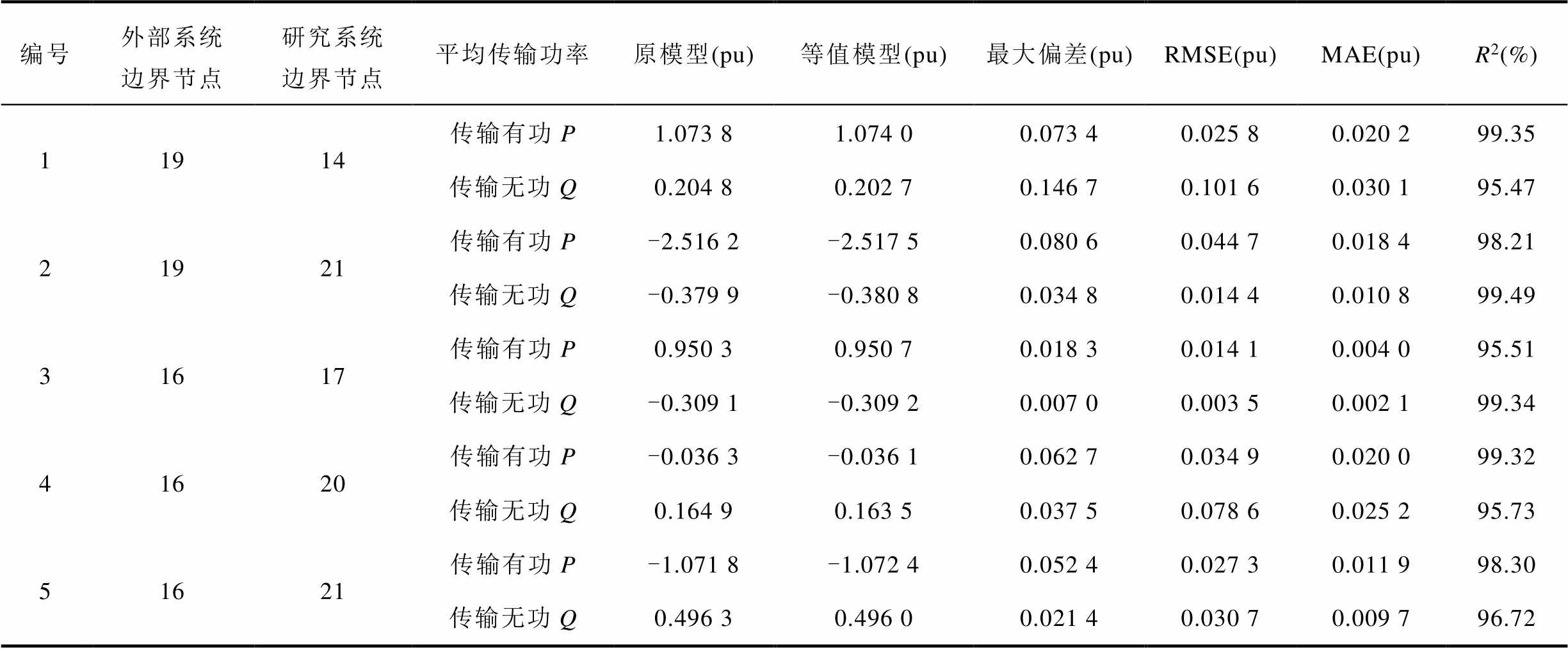
编号外部系统边界节点研究系统边界节点平均传输功率原模型(pu)等值模型(pu)最大偏差(pu)RMSE(pu)MAE(pu)R2(%) 11914传输有功P1.073 81.074 00.073 40.025 80.020 299.35 传输无功Q0.204 80.202 70.146 70.101 60.030 195.47 21921传输有功P-2.516 2-2.517 50.080 60.044 70.018 498.21 传输无功Q-0.379 9-0.380 80.034 80.014 40.010 899.49 31617传输有功P0.950 30.950 70.018 30.014 10.004 095.51 传输无功Q-0.309 1-0.309 20.007 00.003 50.002 199.34 41620传输有功P-0.036 3-0.036 10.062 70.034 90.020 099.32 传输无功Q0.164 90.163 50.037 50.078 60.025 295.73 51621传输有功P-1.071 8-1.072 40.052 40.027 30.011 998.30 传输无功Q0.496 30.496 00.021 40.030 70.009 796.72
由表2计算可得,算例系统等值模型与原模型五条联络线输出有功功率P和无功功率Q拟合精度分别为99.35%、95.47%、98.21%、99.49%、95.51%、99.34%、99.32%、95.73%、98.30%、96.72%,平均模型精度为97.74%,满足实际工程精度要求,可以用来代替外部系统进行动态稳定分析。
模型误差来源分析:
1)Koopman算子截断误差。在实际工程计算中,需要对无限维算子 进行低维辨识,因此会引入低维辨识误差,但通过控制
 算子的阶数可以减小辨识误差,因此该误差可控。
2)模型累计误差。通过Koopman方式对系统升维使系统变成全局线性化系统。但由于对 算子的低维近似辨识,整个系统是近似线性系统。因此在使用最小二乘估计输出系数矩阵时存在模型误差。对于模型长期累计计算,可能会产生模型误差累计,通过增加采样数据可以提高辨识准确度,减小误差。附录第4节证明了这两种误差的收敛可控性。
本节对测量信号加入随机白噪声,验证等值模型在测量数据含噪声时的等值效果。
图15和图16给出了测量信号在噪声影响下等值模型的状态和输出的响应结果,信号信噪比(Signal to Noise Ratio, SNR)为15 dB。由图15和图16可以看出,等值模型较好地滤除了噪声模态,保留了系统动态特性真实模态,在测量数据含噪声时能够准确还原系统动态特性,说明模型具有较好的鲁棒性。
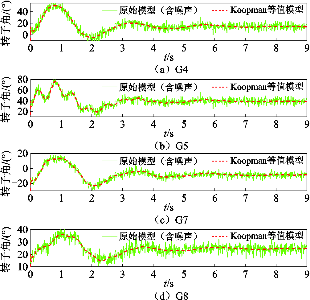
图15 噪声影响下状态方程等值效果
Fig.15 Equivalence effect of state equation under noise
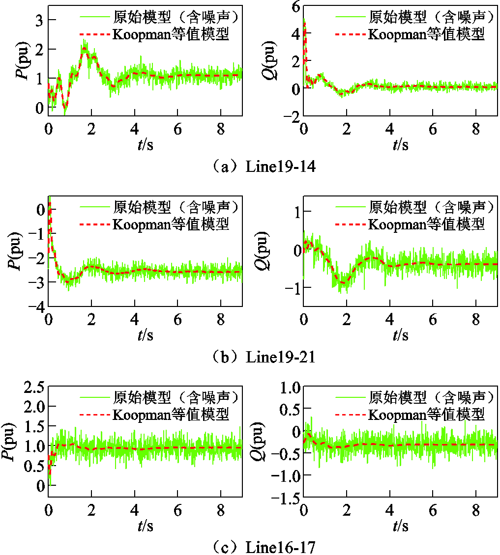
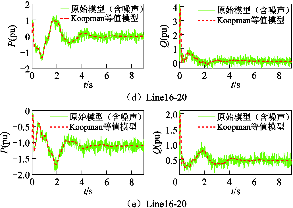
图16 噪声影响下输出方程等值效果
Fig.16 Equivalence effect of output equation under noise
本节选择传统模态方法和同调方法与所提方法进行对比,判断几种模型在模型普适性、建模工作量方面的差异。
1)模型普适性
模态方法基于电力系统运行平衡点的近似线性化模型进行分析,在大扰动下,如短路故障或大型负荷突变,电力系统的动态行为会变得高度非线性,不满足基于系统运行平衡点进行线性化的条件,因此只适用于小扰动下的电力系统动态等值,不适用于大扰动下的电力系统等值。
同调方法通过识别并聚合具有相似或一致动态特性的发电机群,从而简化电力系统的模型。在小扰动下,系统动态特性变化不明显,不能较好地识别并聚合同调发电机群,因此同调方法只适用于大扰动下的电力系统等值。
所提Koopman方法通过无限维线性算子完整地保留了原始系统非线性动态特性,无工作点限制。附录第1节证明了对于任何系统,其高维线性等值Koopman算子的存在。因此对于电网不同的运行方式,都可以通过升维方式实现系统线性化,故所提模型具有更好的普适性。
2)建模工作量
传统模态方法和同调方法均属于机理建模方法。在建模过程中,模态方法和同调方法均需要明确系统详细的内部运行参数数据,在外部系统详细参数不易获取时无法应用。并且等值发电机的分群和聚合过程极为复杂,在外部系统规模较大时,工作量巨大,建模难度高。所提方法基于数据驱动方式,采集等值区域边界数据对模型参数进行辨识,数据容易获取,故建模工作量小。
本文提出了一种电力系统Koopman动态等值模型,对不同程度扰动下的电力系统动态等值方法进行了统一,以增强等值方法对电力系统不确定性和时变运行工况的适应能力,并经算例验证得到如下结论:
1)所提模型基于高维线性Koopman算子完整保留了原始系统的非线性动态特性,避免了基于运行平衡点的模型近似线性化,因此模型无运行工作点限制,适用于不同程度扰动下的电力系统动态等值,提高了电力系统等值模型的鲁棒性和普适性。
2)基于系统边界实测数据辨识等值模型参数,并在测量数据含噪声时对模型参数进行修正,提高了模型的抗噪能力。因此所提方法无需明确系统详解结构和运行参数,减少了对系统内部进行详细建模而带来的工作量。
3)通过算例验证了所提等值模型对系统边界联络线输出功率的响应效果。结果表明,在大扰动和小扰动下,所提Koopman模型与原系统具有基本一致的功角摇摆曲线和功率输出曲线,模型精度为97.74%,能够代替原系统进行动态稳定分析。
附 录
1. 离散可测系统Koopman算子 存在性证明
存在性证明
1)有界性证明
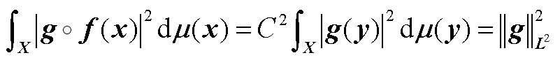
选择观测空间f为二次方可积函数空间 ,其中
,其中 为x上的概率测度,且满足f对的不变性
 (A1)
(A1)
式中, 。此条件确保
 仍属于。
仍属于。
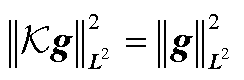
证明是上的有界算子,即
 (A2)
(A2)
代换 得
得
 (A3)
(A3)
取 可得
可得
 (A4)
(A4)
因此可证明是等距算子,即有界。
2)线性证明
由定义直接可得
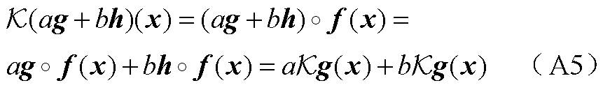
因此证明是线性算子。由以上两点表明,在f保持测度 不变和观测函数空间为
 条件下,存在线性有界Koopman算子满足
 (A6)
(A6)
这表明,对于任何离散可测系统,总能找到一个在高维空间中定义的线性Koopman算子来描述原始系统的动态行为。
2.  和
和 状态空间关系一致性证明
假设式(A7)是系统 的时序状态数据。
 (A7)
(A7)
系统DMD特征矩阵A可表示为
 (A8)
(A8)
考虑m个观测值的集合
 (A9)
(A9)
式中, ;
; 。
。
设 是特征值为
是特征值为 的Koopman算子的特征函数,因此有
 (A10)
(A10)
式中, 。如果
。如果 ,其中R为维度空间,Y的列由
 给出,那么w为特征值为的Koopman算子的左特征向量,因此有
 (A11)
(A11)
这表明,如果:①提供动态模式分解的观测集足够多,满足 ;②数据足够丰富,满足
 ,就可以说明动态模式分解算法辨识的
 和
和 具有相同的状态空间特性。通过采集足够多的数据,可以辨识出
 的低维等效算子
 ,其具有相同的特征值和特征函数,可以代替原空间进行谱分解。
3. 模型收敛性证明
定义由观测函数张成的空间 为Koopman算子
 的不变子空间,其协方差矩阵可表示为
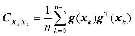 (A12)
(A12)
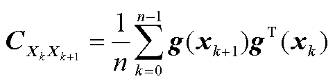 (A13)
(A13)
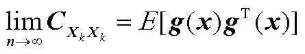
由遍历性定理可得,当 时,有
时,有
 (A14)
(A14)
 (A15)
(A15)
 可写为
可写为
 (A16)
(A16)
因此当时,收敛到 ,即
,即
 (A17)
(A17)
式(A17)即为Koopman算子在不变子空间 上的投影。即当时,DMD的估计处收敛到在不变子空间上的投影矩阵。由附录第1节可得存在且有界,因此等值模型收敛。
4. 模型误差收敛性证明
1)截断误差收敛证明
定义 在希尔伯特空间中的SVD为
 (A18)
(A18)
式中, 为奇异值;
为奇异值; 、
、 为奇异向量。
根据Eckart-Young定理,截断误差满足
 (A19)
(A19)
截断误差由第r+1个奇异值决定,由于系统每个模态间能量是衰减的,满足 ,因此模型截断误差收敛。
2)累计误差收敛证明
定义模型第k次预测误差为
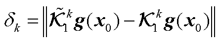 (A20)
(A20)
基于三角不等式和算子范数性质,有
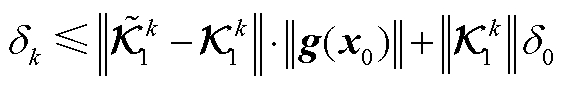 (A21)
(A21)
进一步分解 为
为
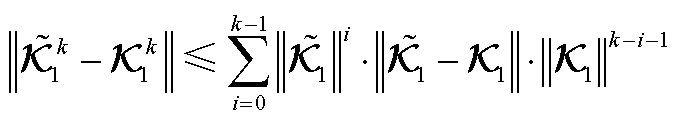 (A22)
(A22)
若 且
且 ,则长期累计误差满足
 (A23)
(A23)
式中, ,
, 为矩阵谱半径;C为与维度相关系数;e为误差界限常数。
这表明,对于稳定的系统, ,系统长期累计误差随k按指数迅速衰减,因此模型长期累计误差收敛。
5. 演化系数b的计算方法
数据矩阵可分解为
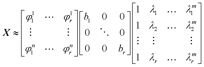 (A24)
(A24)
式中, 为系统模态;n为系统状态数;m为观测序列数;r为保留奇异值数。
b可由式(A25)求解。
 (A25)
(A25)
式中, ,Y为的左特征向量;Db为构造的系统振幅矩阵;Vand为特征值迭代的范德蒙矩阵。将X的SVD结果和式(A25)联立得
 (A26)
(A26)
定义误差函数为
 (A27)
(A27)
可得演化系数b的计算结果为
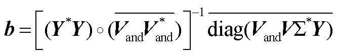 (A28)
(A28)
6. 不同扰动下算例系统动态等值结果
大扰动和小扰动下算例系统Koopman动态等值方程结果为
 (A29)
(A29)
大扰动下系数矩阵辨识结果见附表1、附表2。小扰动下系数矩阵辨识结果见附表3、附表4。
附表1 大扰动下外部系统状态系数矩阵辨识结果
App.Tab.1 Identification results of the state coefficient matrix of the external system under large disturbances
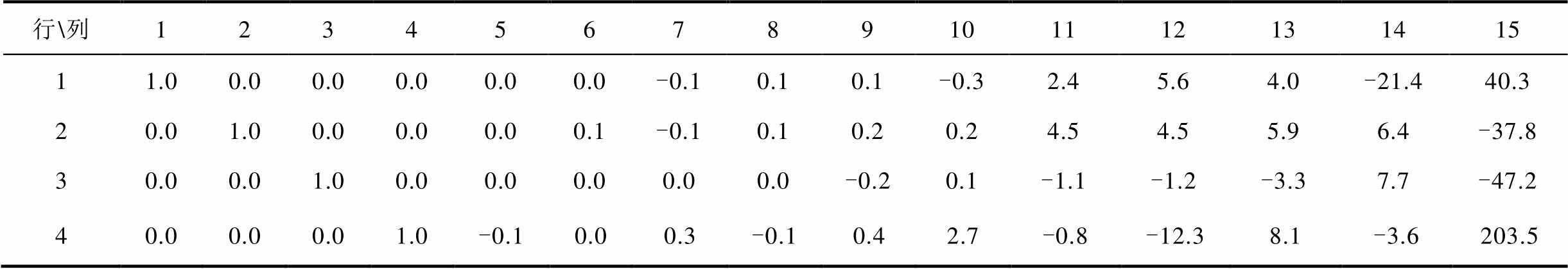
行\列123456789101112131415 11.00.00.00.00.00.0-0.10.10.1-0.32.45.64.0-21.440.3 20.01.00.00.00.00.1-0.10.10.20.24.54.55.96.4-37.8 30.00.01.00.00.00.00.00.0-0.20.1-1.1-1.2-3.37.7-47.2 40.00.00.01.0-0.10.00.3-0.10.42.7-0.8-12.38.1-3.6203.5
(续)
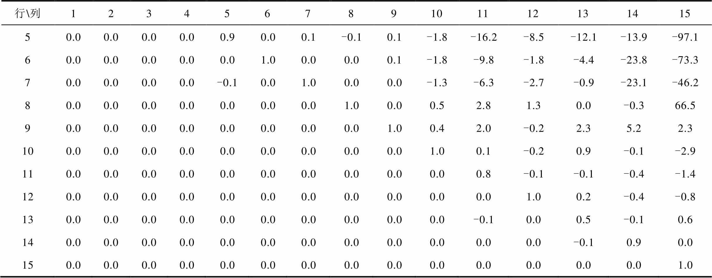
行\列123456789101112131415 50.00.00.00.00.90.00.1-0.10.1-1.8-16.2-8.5-12.1-13.9-97.1 60.00.00.00.00.01.00.00.00.1-1.8-9.8-1.8-4.4-23.8-73.3 70.00.00.00.0-0.10.01.00.00.0-1.3-6.3-2.7-0.9-23.1-46.2 80.00.00.00.00.00.00.01.00.00.52.81.30.0-0.366.5 90.00.00.00.00.00.00.00.01.00.42.0-0.22.35.22.3 100.00.00.00.00.00.00.00.00.01.00.1-0.20.9-0.1-2.9 110.00.00.00.00.00.00.00.00.00.00.8-0.1-0.1-0.4-1.4 120.00.00.00.00.00.00.00.00.00.00.01.00.2-0.4-0.8 130.00.00.00.00.00.00.00.00.00.0-0.10.00.5-0.10.6 140.00.00.00.00.00.00.00.00.00.00.00.0-0.10.90.0 150.00.00.00.00.00.00.00.00.00.00.00.00.00.01.0
附表2 大扰动下外部系统输出系数矩阵 辨识结果
辨识结果
App.Tab.2 Identification results of the output coefficient matrix  of the external system under large disturbances

行\列123456789101112131415 10.00.00.00.00.10.00.7-0.725.7-3.023.1-400.6363.4-35.426.1 20.0-0.10.00.0-0.30.1-1.51.6-7.5-14.76.01 060.1-2723.7158.01526.3 30.00.00.00.00.10.00.7-0.76.17.620.7-388.7584.2-42.7-188.4 40.0-0.1-0.10.0-0.10.1-1.41.510.2-18.8-74.5598.2-906.677.1318.2 50.00.00.00.0-0.10.1-1.01.1-19.0-5.2-29.4682.7-745.062.757.2 60.0-0.2-0.10.1-0.70.4-7.47.7-102.3-53.5-223.93 335.5-3 364.7352.776.1 70.00.00.00.0-0.10.0-0.60.6-2.9-7.232.4207.7-681.847.5405.7 80.00.00.00.00.00.00.3-0.33.50.422.4-83.2-228.31.6282.9 90.0-0.2-0.10.1-0.60.3-6.87.1-84.8-47.6-216.02 981.4-2 681.6294.3-230.3 100.0-0.1-0.10.0-0.20.1-2.22.4-30.0-17.5-85.81026.3-1 063.2104.172.1
附表3 小扰动下外部系统状态系数矩阵 辨识结果
辨识结果
App.Tab.3 Identification results of the state coefficient matrix of the external system under small disturbances
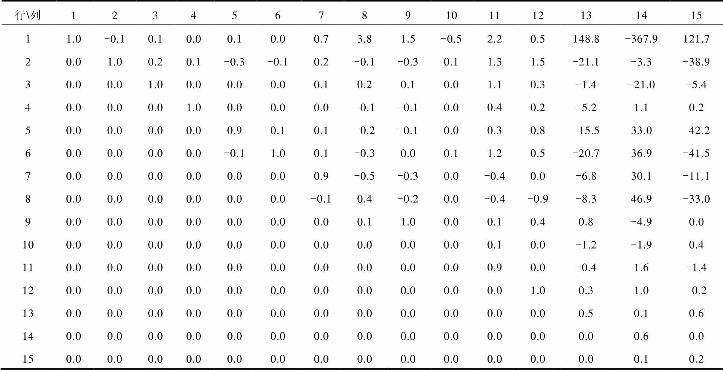
行\列123456789101112131415 11.0-0.10.10.00.10.00.73.81.5-0.52.20.5148.8-367.9121.7 20.01.00.20.1-0.3-0.10.2-0.1-0.30.11.31.5-21.1-3.3-38.9 30.00.01.00.00.00.00.10.20.10.01.10.3-1.4-21.0-5.4 40.00.00.01.00.00.00.0-0.1-0.10.00.40.2-5.21.10.2 50.00.00.00.00.90.10.1-0.2-0.10.00.30.8-15.533.0-42.2 60.00.00.00.0-0.11.00.1-0.30.00.11.20.5-20.736.9-41.5 70.00.00.00.00.00.00.9-0.5-0.30.0-0.40.0-6.830.1-11.1 80.00.00.00.00.00.0-0.10.4-0.20.0-0.4-0.9-8.346.9-33.0 90.00.00.00.00.00.00.00.11.00.00.10.40.8-4.90.0 100.00.00.00.00.00.00.00.00.00.00.10.0-1.2-1.90.4 110.00.00.00.00.00.00.00.00.00.00.90.0-0.41.6-1.4 120.00.00.00.00.00.00.00.00.00.00.01.00.31.0-0.2 130.00.00.00.00.00.00.00.00.00.00.00.00.50.10.6 140.00.00.00.00.00.00.00.00.00.00.00.00.00.60.0 150.00.00.00.00.00.00.00.00.00.00.00.00.00.10.2
附表4 小扰动下外部系统输出系数矩阵 辨识结果
辨识结果
App.Tab.4 Identification results of the output coefficient matrix  of the external system under small disturbances
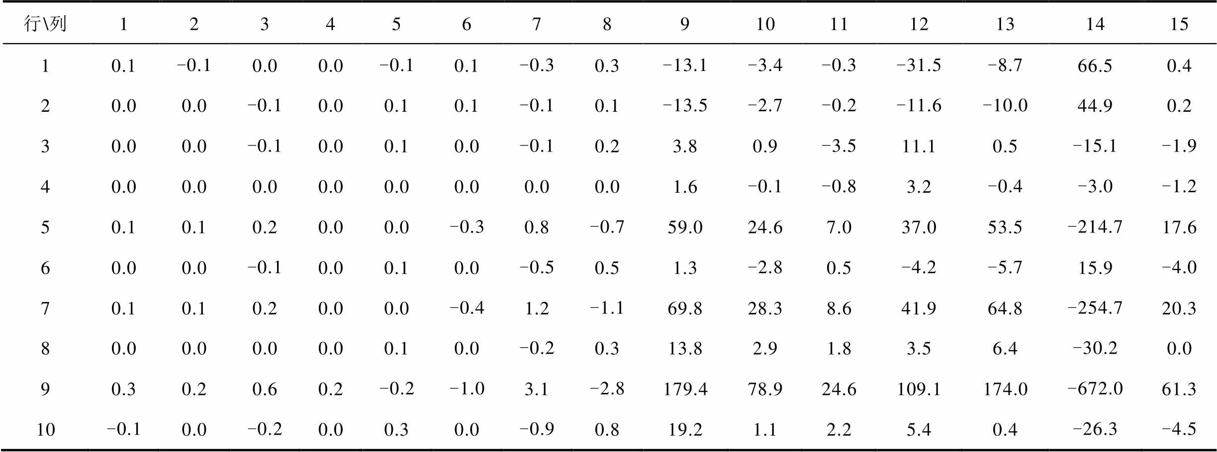
行\列123456789101112131415 10.1-0.10.00.0-0.10.1-0.30.3-13.1-3.4-0.3-31.5-8.766.50.4 20.00.0-0.10.00.10.1-0.10.1-13.5-2.7-0.2-11.6-10.044.90.2 30.00.0-0.10.00.10.0-0.10.23.80.9-3.511.10.5-15.1-1.9 40.00.00.00.00.00.00.00.01.6-0.1-0.83.2-0.4-3.0-1.2 50.10.10.20.00.0-0.30.8-0.759.024.67.037.053.5-214.717.6 60.00.0-0.10.00.10.0-0.50.51.3-2.80.5-4.2-5.715.9-4.0 70.10.10.20.00.0-0.41.2-1.169.828.38.641.964.8-254.720.3 80.00.00.00.00.10.0-0.20.313.82.91.83.56.4-30.20.0 90.30.20.60.2-0.2-1.03.1-2.8179.478.924.6109.1174.0-672.061.3 10-0.10.0-0.20.00.30.0-0.90.819.21.12.25.40.4-26.3-4.5
参考文献
[1] 王淏, 谢开贵, 邵常政, 等. 柔性互联输配一体化电网有损潮流的精细化建模及应用[J]. 电工技术学报, 2024, 39(9): 2593-2607. Wang Hao, Xie Kaigui, Shao Changzheng, et al. Precise lossy power flow modeling and application of integrated transmission and distribution grids with multi-terminal flexible interconnected[J]. Transactions of China Electrotechnical Society, 2024, 39(9): 2593-2607.
[2] 王力, 胡佳成, 曾祥君, 等. 基于混合储能的交直流混联微电网功率分级协调控制策略[J]. 电工技术学报, 2024, 39(8): 2311-2324. Wang Li, Hu Jiacheng, Zeng Xiangjun, et al. Hierarchical coordinated power control strategy for AC-DC hybrid microgrid with hybrid energy storage[J]. Transactions of China Electrotechnical Society, 2024, 39(8): 2311-2324.
[3] 刘宿城, 褚勇智, 刁吉祥, 等. 基于输入-状态稳定条件的直流微电网集群分布式大信号稳定性[J]. 电工技术学报, 2025, 40(2): 544-558. Liu Sucheng, Chu Yongzhi, Diao Jixiang, et al. Distributed large signal stability based on input-to-state stability conditions for DC microgrid clusters[J]. Transactions of China Electrotechnical Society, 2025, 40(2): 544-558.
[4] 陈昆明, 马成斌. 基于DIgSILENT的风电场等值建模研究[J]. 电气技术, 2020, 21(4): 15-19, 75. Chen Kunming, Ma Chengbin. Research on wind farm equivalent modeling based on DIgSILENT[J]. Electrical Engineering, 2020, 21(4): 15-19, 75.
[5] 刘光晔, 杨以涵. 电力系统电压稳定与功角稳定的统一分析原理[J]. 中国电机工程学报, 2013, 33(13): 135-149. Liu Guangye, Yang Yihan. Theoretical foundation of power system voltage and angle stability unified analysis[J]. Proceedings of the CSEE, 2013, 33(13): 135-149.
[6] 郭孟杰, 杜文娟, 王海风. 直驱风电场单机等值模型下次/超同步振荡模式特征的准确度分析与评价[J]. 电网与清洁能源, 2024, 40(9): 105-113. Guo Mengjie, Du Wenjuan, Wang Haifeng. Accuracy analysis and evaluation of sub/super-synchronous oscillation mode characteristics of PMSG-based wind farm single-machine equivalent models[J]. Power System and Clean Energy, 2024, 40(9): 105-113.
[7] 潘学萍, 王卫康, 陈海东, 等. 计及低电压穿越影响的感应电动机动态分群[J]. 电工技术学报, 2024, 39(7): 2001-2016, 2032. Pan Xueping, Wang Weikang, Chen Haidong, et al. Study of dynamic clustering method for induction motors considering low voltage ride through effects[J]. Transactions of China Electrotechnical Society, 2024, 39(7): 2001-2016, 2032.
[8] 潘学萍, 张弛, 鞠平, 等. 风电场同调动态等值研究[J]. 电网技术, 2015, 39(3): 621-627. Pan Xueping, Zhang Chi, Ju Ping, et al. Coherency-based dynamic equivalence of wind farm composed of doubly fed induction generators[J]. Power System Technology, 2015, 39(3): 621-627.
[9] 罗佳奕, 韩蓓, 徐晋, 等. 基于松弛变异系数的多微电网同调判定与等值建模[J]. 电力系统自动化, 2023, 47(17): 67-74. Luo Jiayi, Han Bei, Xu Jin, et al. Homology identification and equivalent modelling of multi-microgrid based on relaxed variation coefficients[J]. Automation of Electric Power Systems, 2023, 47(17): 67-74.
[10] 李高望, 张智, 李达, 等. 基于Prony分析特征提取的同调机组分群方法[J]. 电力系统保护与控制, 2020, 48(22): 91-99. Li Gaowang, Zhang Zhi, Li Da, et al. Coherency clustering method based on Prony analysis feature extraction[J]. Power System Protection and Control, 2020, 48(22): 91-99.
[11] 廖庭坚, 刘光晔, 雷强, 等. 计及电动机负荷的电力系统动态等值分析[J]. 电网技术, 2016, 40(5): 1442-1446. Liao Tingjian, Liu Guangye, Lei Qiang, et al. Analysis of dynamic equivalence with consideration of motor loads in power systems[J]. Power System Technology, 2016, 40(5): 1442-1446.
[12] 李秀全, 邵玉槐, 张强. 电力系统同调动态等值的应用[J]. 电气技术, 2008, 9(2): 34-36. Li Xiuquan, Shao Yuhuai, Zhang Qiang. Application of coherency-based dynamic equivalence[J]. Electrical Engineering, 2008, 9(2): 34-36.
[13] 洪国庆, 吴国旸, 金宇清, 等. 电力系统风力发电建模与仿真研究综述[J]. 电力系统自动化, 2024, 48(17): 22-36. Hong Guoqing, Wu Guoyang, Jin Yuqing, et al. Review on research of modeling and simulation for wind power generation in power system[J]. Automation of Electric Power Systems, 2024, 48(17): 22-36.
[14] 姜涛, 张明宇, 李雪, 等. 基于正交子空间投影的电力系统同调机群辨识[J]. 电工技术学报, 2018, 33(9): 2077-2088. Jiang Tao, Zhang Mingyu, Li Xue, et al. Estimating coherent generators from measurement responses in power systems using orthogonal subspace projection [J]. Transactions of China Electrotechnical Society, 2018, 33(9): 2077-2088.
[15] 王进钊, 严干贵, 刘侃. 基于交替方向隐式平衡截断法的直驱风电场次同步振荡分析的模型降阶研究[J]. 发电技术, 2023, 44(6): 850-858. Wang Jinzhao, Yan Gangui, Liu Kan. Research on model reduction of direct drive wind farm subsynchronous oscillation analysis based on alternating direction implicit balanced truncation method[J]. Power Generation Technology, 2023, 44(6): 850-858.
[16] 韩平平, 方佳维, 丁明, 等. 利用特征值分析法的双馈风电机组模型降阶[J]. 电力系统及其自动化学报, 2017, 29(8): 8-14. Han Pingping, Fang Jiawei, Ding Ming, et al. Simplification of DFIG models with eigenvalue analysis[J]. Proceedings of the CSU-EPSA, 2017, 29(8): 8-14.
[17] 王玉鹏, 严干贵, 杨成, 等. 风电并网系统次同步等幅振荡机理与特性分析[J]. 华中科技大学学报(自然科学版), 2024, 52(7): 45-51. Wang Yupeng, Yan Gangui, Yang Cheng, et al. Mechanism and characteristics analysis of sub-synchronous constant amplitude oscillation in wind power grid connected systems[J]. Journal of Huazhong University of Science and Technology (Natural Science Edition), 2024, 52(7): 45-51.
[18] 刘铖, 赵晓洋, 张宇驰, 等. 面向区域间振荡模式的电力系统小扰动惯量域构建[J]. 电力系统保护与控制, 2021, 49(20): 9-19. Liu Cheng, Zhao Xiaoyang, Zhang Yuchi, et al. Construction of a small signal inertia region of a power system for inter-area oscillation mode[J]. Power System Protection and Control, 2021, 49(20): 9-19.
[19] 李戎, 李建文, 李永刚, 等. 结合特征[根及模态分析法的逆变器多机并网系统谐波扰动响应分析[J]. 电工技术学报, 2024, 39(14): 4519-4534. Li Rong, Li Jianwen, Li Yonggang, et al. Analysis of harmonic disturbance response of multi-inverter grid-connected system combining characteristic root and modal analysis method[J]. Transactions of China Electrotechnical Society, 2024, 39(14): 4519-4534.
[20] 彭天海, 蔡萱, 瞿子涵, 等. 计及大规模电网分级分区解耦的区域电网供电碳排放因子计算模型研究[J]. 中国电机工程学报, 2024, 44(3): 894-905. Peng Tianhai, Cai Xuan, Qu Zihan, et al. Research on calculation model of power supply carbon emission factor in regional power grid considering hierarchical and regional decoupling of large-scale power grid[J]. Proceedings of the CSEE, 2024, 44(3): 894-905.
[21] 马燕峰, 程有深, 赵书强, 等. 双馈风电场并网引起火电机组多模态次同步谐振机理分析[J]. 电工技术学报, 2025, 40(5): 1395-1410. Ma Yanfeng, Cheng Youshen, Zhao Shuqiang, et al. Mechanism analysis of multi-mode SSR of thermal power unit caused by doubly fed wind farm integration[J]. Transactions of China Electrotechnical Society, 2025, 40(5): 1395-1410.
[22] Donoho D L. De-noising by soft-thresholding[J]. IEEE Transactions on Information Theory, 1995, 41(3): 613-627.
[23] Dawson S T M, Hemati M S, Williams M O, et al. Characterizing and correcting for the effect of sensor noise in the dynamic mode decomposition[J]. Experiments in Fluids, 2016, 57(3): 42.
Abstract There is a lack of dynamic equivalent modeling methods for power systems that can be applied to both large and small disturbances. To enhance the adaptability of the equivalence method to uncertainties and time-varying operating conditions in power systems, a Koopman dynamic equivalence method for power systems under different levels of disturbance is proposed, which unifies the dynamic equivalence methods for power systems under different operating conditions.
First, establish the state space equation of the external system, perform high-dimensional linearization mapping based on the Koopman operator, and establish its global linearized equivalent model in high-dimensional space. Through this mathematical mapping, the model is linearized without losing key information, so the model is applicable to all operating conditions of the power system.
Then, based on the data-driven approach, the parameters of the equivalent model are identified by collecting equivalent boundary data. The dynamic mode decomposition (DMD) and least squares are used to identify the state coefficient matrix and output coefficient matrix of the equivalent model, respectively. When the measurement data contains noise, the model parameters are adjusted using least squares dynamic mode decomposition (LS-DMD) and total least squares (TLS) to enhance the model's noise resistance. This process does not require explicit system detailed structure and operating parameters, thus reducing the workload of detailed modeling. The low-dimensional identification DMD matrix of the external system's state coefficient matrix  shares the same state-space characteristics with the original matrix. Therefore, the numerical solution for the state of the original model can be obtained through the spectral decomposition of the DMD matrix.
Then, the Koopman modes are extracted by spectral decomposition of the system state coefficient matrix. The mode with eigenvalues closer to the imaginary axis has a greater impact on the system and will dominate the dynamic characteristics of the system. The rapidly decaying modes have a relatively small impact on the dynamic characteristics of the system. By retaining the analysis of modes that have a greater impact on the system and filtering out rapidly decaying modes, it is possible to achieve reduced order of the equivalent model and significantly reduce the computational load.
Finally, the proposed method is tested on examples of external systems experiencing transient (large disturbances) and steady-state (small disturbances), respectively. The results show that the proposed equivalent model has basically consistent power angle swing curves and equivalent boundary tie line power output curves with the original system, regardless of whether the system is under large or small disturbances. Quantitative analysis was conducted under large disturbance cases, and the fitting accuracy of the equivalent model and the original model for the transmission of active and reactive power on the five tie lines was 99.35%, 95.47%, 98.21%, 99.49%, 95.51%, 99.34%, 99.32%, 95.73%, 98.30%, and 96.72%, respectively, with an average model accuracy of 97.74%.
The following conclusions are obtained through the verification of the examples: (1) The proposed model, based on the high-dimensional linear Koopman operator, fully preserves the nonlinear dynamic characteristics of the original system. So the model has no restrictions on operating points and is suitable for dynamic equivalence of power systems under varying degrees of disturbance, enhancing the robustness and universality of power system equivalence models. (2) The parameters of the equivalent model are identified based on the measured data of the system boundary, so the proposed method does not require explicit detailed structural and operational parameters of the system, reducing the workload associated with detailed modeling of the internal structure of the system. (3) The effectiveness of the proposed equivalent model was verified through examples. The results show that the proposed model has basically the same power angle swing curve and power output curve as the original system under large and small disturbances, with a model accuracy of 97.74%. The model can replace the original system for dynamic stability analysis under different levels of disturbance.
keywords:Dynamic equivalence, Koopman, modal method, homology method, different disturbance
DOI: 10.19595/j.cnki.1000-6753.tces.242346
中图分类号:TM74
国家电网有限公司总部管理科技项目资助(5100-202355409A-3-2-ZN)。
收稿日期 2024-12-26
改稿日期 2025-02-22
张子傲 男,2000年生,硕士研究生,研究方向为新能源电力系统分析与控制。E-mail:zhangdabei1717@163.com
刘 君 女,1970年生,副教授,研究方向为电力系统分析与控制、先进输变电技术、新能源电力系统特性与多源互补等。E-mail:liujunlishu@126.com(通信作者)
(编辑 赫 蕾)