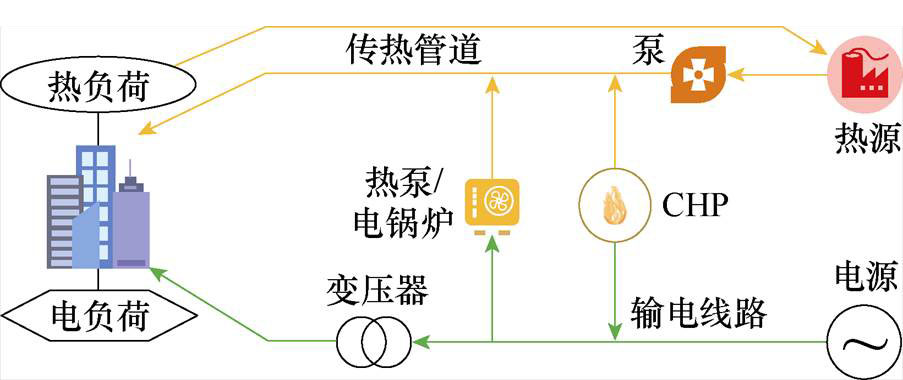
图1 电热综合能源系统结构
Fig.1 Electrothermal integrated energy system structure diagram
摘要 为实现多种能源互补共济与高效利用,集多种异质能源于一体的综合能源系统受到了广泛的关注。而综合能源系统的动态能流计算对后续的优化控制与能源调度研究起着重要作用。为了精准地描述热力网络的动态特性,实现对综合能源系统的连续动态能流计算,该文提出一种基于全纯嵌入的电热综合能源系统动态能流联合计算方法。首先,对热网动态模型做空间离散化处理,保留温度对时间的微分,将热力网络的偏微分动态方程转化常微分方程。其次,利用时变的全纯函数对电-热能流方程进行重构,构建全纯嵌入的电-热动态能流模型,并递归求解全纯函数的系数,得到能流的解析表达式。最后,先用单个热力管道算例验证模型的有效性和准确性,而后用IEEE 14节点标准算例和51节点热力网络耦合成的电热互联系统算例进行仿真分析,设置热负荷、电负荷和发电机出力发生波动的场景,并将仿真结果与分解求解法、快速灵活全纯嵌入法、龙格库塔法进行对比。仿真结果表明,该文所提方法可获得准确、连续的动态能流解,同时能够精准地描述能流响应扰动的过程。
关键词:全纯嵌入法 能流计算 动态仿真 递归计算
为应对日益凸显的能源危机和环境污染问题,我国提出“碳达峰、碳中和”战略目标。综合能源系统(Integrated Energy System, IES)耦合了多种能源网络,在实现不同能源互补互济的同时,可以提高能源的利用效率。目前,针对IES的研究主要围绕多能耦合建模、规划设计和优化运行展开,而IES能流计算分析是开展上述研究的重要基础[1-2]。
目前,有部分学者建立IES的稳态模型实现快速多能流计算。文献[3]建立了电网与天然气网耦合运行时的稳态多能流模型。文献[4]建立了电热综合能源系统的稳态快速计算模型。文献[5]将水力计算的节点法和回路法应用于电-气综合能流计算。文献[6]研究了计及氢气注入的电-热-气IES稳态混合能流计算。文献[7]进一步考虑了时间尺度特性,提出了多能流准稳态的计算模型,解决了传统多能流算法对初值较为敏感的问题。文献[8]考虑天然气传输的慢时间特性,建立了电-气统一潮流模型,可以分析电-气综合能源系统的耦合作用机理。文献[9]则进一步考虑传输延时,采用节点法将管道出口温度表征为若干水块温度的线性组合。上述IES稳态模型的建模及求解无法在负荷或出力发生波动的场景下反映多能流受扰动的过程,且部分算法迭代次数较多,计算效率一般。
此外,还有部分学者对IES的动态模型进行简化处理,或者使用间接求解方法开展动态能流计算。文献[10]采用有限差分法描述热流的动态分布。而文献[11-12]在此基础上优化了差分步长和差分格式,提高了模型的精度与效率。进一步地,文献[13-14]提出了以拉普拉斯变换为基础的广义电路统一建模方法,将时域的复杂网络关系转化为拉普拉斯频域电路网络关系,实现了频域下的统一建模。文献[15-16]则提出了直观的统一能路理论,利用傅里叶变换将时域问题映射到频域求解,降低了网络分析的计算复杂度,相比传统方法大大提高了计算效率。文献[17]构建了基于广义时域导纳矩阵的网络统一模型,并根据综合能源各子系统的运行特性推导了不同系统的时域二端口方程。值得注意的是,该模型的精度受离散格式和离散步长的影响,高维场景下求解精度不足。
上述动态能流计算大多基于迭代类方法,而迭代类算法存在收敛速度慢、对初值敏感等问题。为此,文献[18]提出了一种全纯嵌入潮流递归算法(Holomorphic Embedding Method, HEM),将潮流方程转化为全纯函数的形式,实现了对原始非线性方程的线性化处理,简化了求解过程。该方法具有较好的数值稳定性及收敛性[19],目前已有学者将其应用于IES能流计算中。文献[20]提出一种基于全纯嵌入的电-气IES多能流计算方法,采用分解求解(Holomorphic Embedding Factorization Solution, HEFS)法对电力网络和天然气网络分别进行能流计算,但求解过程中需要反复判断子系统能流是否收敛,对于强耦合系统计算效率不高。文献[21]提出了一种基于全纯嵌入的快速灵活IES能流(Fast and Flexible Holomorphic Embedding, FFHE)算法。该方法根据电力网络、供热网络和天然气网络的稳态方程确定各网络的递推方程,从而得到统一的全纯嵌入递归解形式,但此方法对热网及气网的管道动态特性描述并不清晰,计算得到的仍为时间断面下的能流解。
为进一步提高动态能流计算的精度和效率,实现动态能流的连续求解,本文提出一种基于全纯嵌入的电-热IES动态能流联合计算方法。首先,介绍电热综合能源系统动态模型,并将热网动态模型中温度对空间的微分项差分化;其次,以时间为变量的全纯函数嵌入节点电压及节点温度,重构电-热IES的微分代数方程;最后,采用联合求解(Holomorphic Embedding Sequential Solution, HESS)法,令等式两侧幂级数系数相等实现全纯函数的递归求解,进而得到能流的解析表达式。
电热综合能源系统(Integrated Heat and Electricity Systems, IHES)由电力系统、热力系统和耦合单元三部分组成,如图1所示。电力和热力系统通过耦合单元相互连接,如电锅炉(Electric Boiler, EB)、热泵(Heat Pump, HP)和热电联产机组(Combined Heat and Power, CHP)。
IES中异质能流传输的时间尺度有很大差异。电力系统受到扰动后,可在较短的时间内恢复平衡,而热力系统在受到扰动后需要几十分钟甚至几小时来恢复平衡状态。所以,在电热综合能源系统动态仿真中,电力系统可采用稳态模型[22],而热力系统要利用考虑时间尺度的偏微分方程描述其动态特性。
图1 电热综合能源系统结构
Fig.1 Electrothermal integrated energy system structure diagram
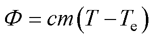
热力系统的动态特性主要体现在热量传递过程中的传输时延和传输热损耗。热网中热流与环境的辐射换热较小,可将其忽略[23]。以环境温度为参考温度,以管道中热流的温度 和热流实际携带的热功率
 为状态量,则状态量之间满足
 (1)
(1)
式中,c为水的比热容[J/(kg·℃)];m为流入管道的热水质量流量(kg/h); 为环境温度(℃)。为方便计算,下文将表示为管道温度和环境温度之间的差值。
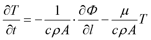
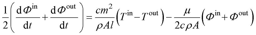
根据能量守恒定律,热力流在管道中的传输过程可以用两个偏微分方程来描述,即
 (2)
(2)
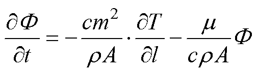 (3)
(3)
式中,l为管道长度(m);t为时间(min); 为水的密度(kg/m3);A为管道横截面积(m2);
 为传热系数[W/(m2·℃)]。
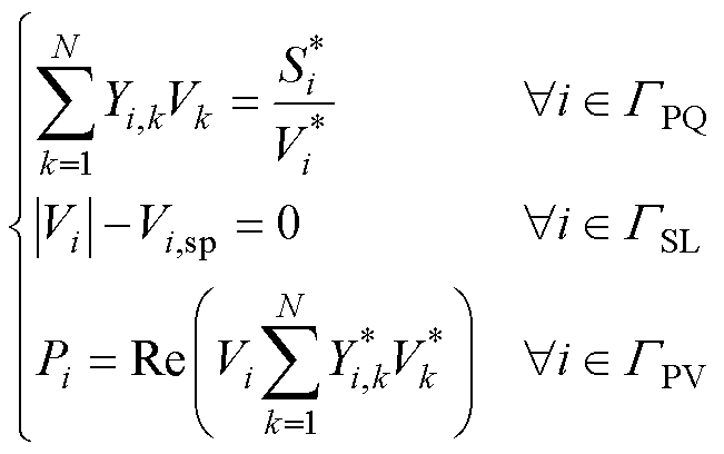
本文利用稳态潮流方程描述电力系统的运行状态[19],即
 (4)
(4)
式中, 为节点导纳矩阵中第
 行第
行第 列的元素;
列的元素; 和
和 为节点电压及其共轭;
 为节点注入的复功率的共轭值;
 和
和 为节点电压及其共轭;
 为PV节点的指定电压幅值;Re表示取复数的实数部分;
 、
、 、
、 分别为PQ节点、PV节点和松弛节点的集合。
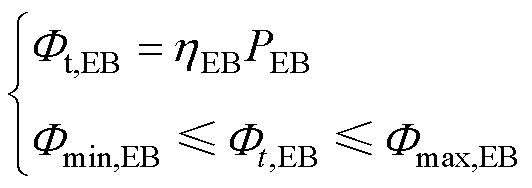
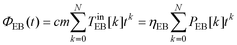
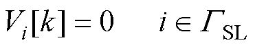
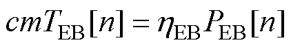
电-热耦合设备包括EB、HP及CHP等。其中,电转热设备HP和EB消耗电能满足热负荷需求,其运行特性可描述为
 (5)
(5)
式中, 为电转热设备的转换效率;
 为电转热设备产热功率;
 为电转热设备产热功率下、上限区间。
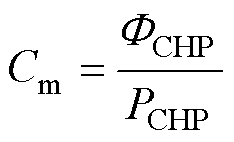
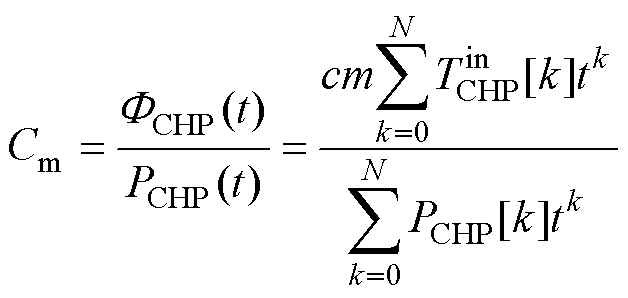
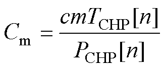
CHP机组既能生产电能,又能利用背压发电机的乏汽进行供热[24],模型为
 (6)
(6)
式中, 为产热产电比;
 为背压机组发出的热功率;
 为背压机组发出的电功率。
1.1节给出了IHES中热网的偏微分形式的动态模型。传统解法是分别对时间和空间的偏微分方程做差分处理,截取时间和空间的断面来进行计算[10]。为了实现对热网动态能流的连续求解,本节在传统方法的基础上,对热网管道只做空间离散化处理,将热网偏微分方程转化为只含对时间微分的常微分方程。
2.1.1 单个供热管道建模
将长度为l的管道划分为N段,每段的长度
 ,热网管道距离差分如图2所示。每段入口和出口处的热流温度分别为
 和
和 。
。
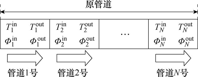
图2 热网管道距离差分
Fig.2 Distance difference of heat supply network pipeline
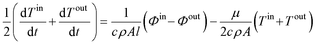
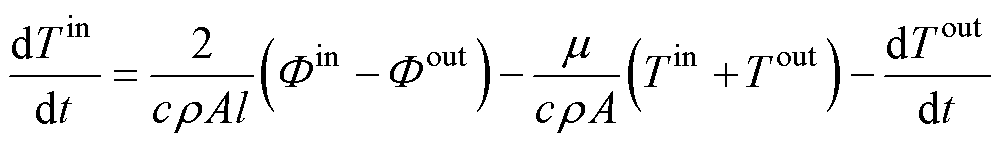
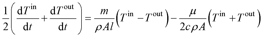
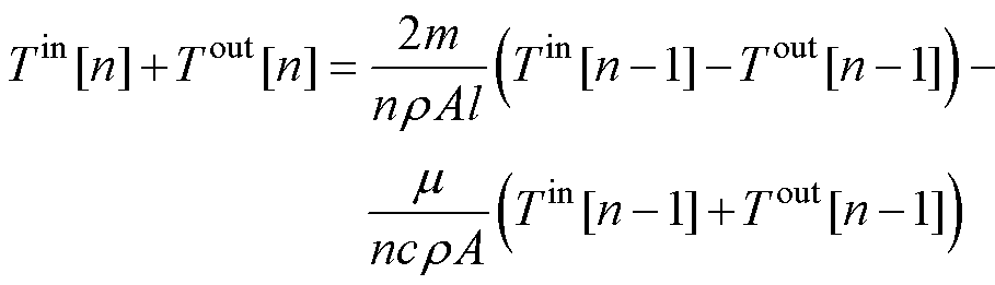
使用梯形积分公式,将式(2)、式(3)中水温和其携带的热功率对距离的偏微分方程,改写为进出口端温度和热功率对管道长度 的差分形式,即
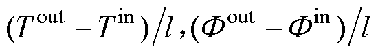 ;而热水的温度和其携带的热功率对时间的偏微分由管道进出口两端温度和热功率对时间微分的平均值代替,即
 。将热网偏微分方程转化为只含对时间微分的常微分方程为
 (7)
(7)
 (8)
(8)
2.1.2 流入同一节点的热网管道建模
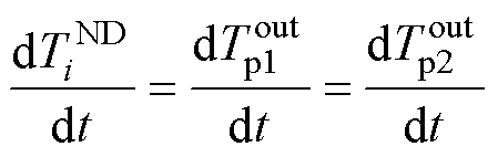
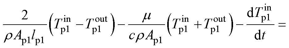
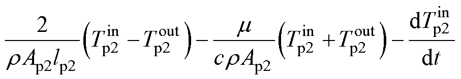
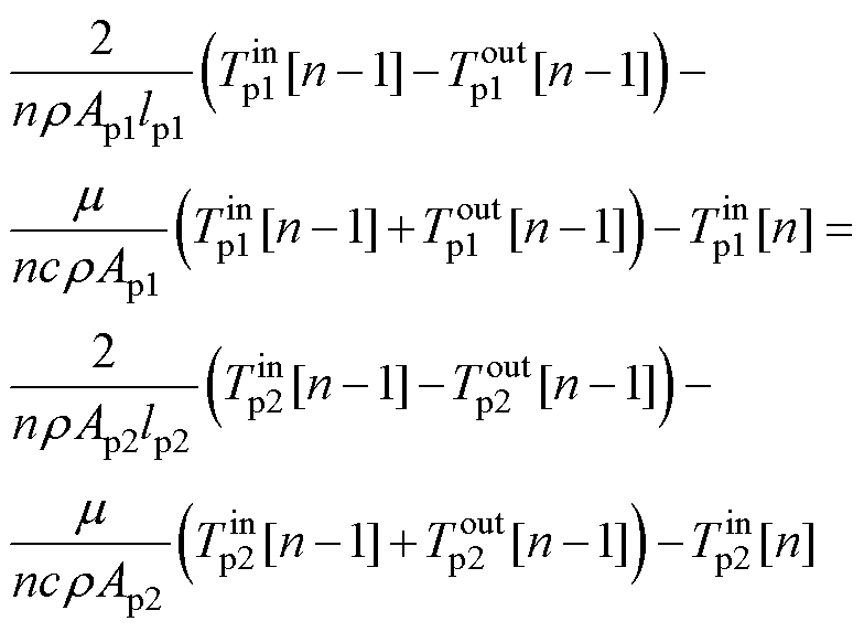
热网中还存在两个甚至两个以上的管道末端汇集于同一节点的情况,这种节点称为“聚合节点”[21]。聚合节点如图3所示,管道p1和p2均流入节点i,则聚合节点i的出口温度和p1、p2管道的末端温度相等,构成了新的约束条件为
 (9)
(9)
式中, 是节点i的温度(℃)。
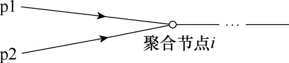
图3 聚合节点
Fig.3 Aggregate node
由此,可将式(7)改写为
 (10)
(10)
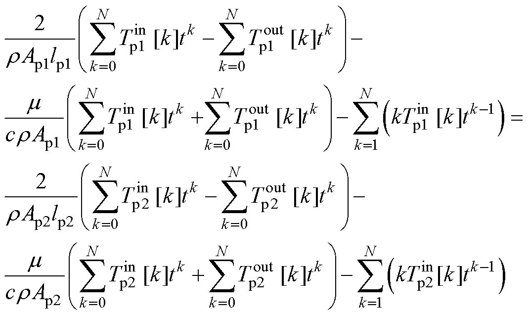
由式(9)和式(10)可得
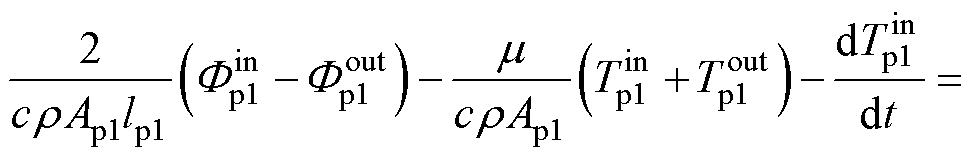
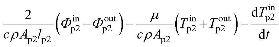 (11)
(11)
式中, 、
、 为管道p1、p2的截面积(m2);
 、
、 为管道p1、p2的长度(m)。
综上所述,热网动态模型的常微分形式可以由式(9)~式(11)表示。
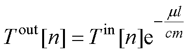
供热系统中常用质调节模式,即在热源处只改变热网的供水温度,保持热流的质量流量m不变的调节方法[25]。则状态量热流温度和其所携带的热功率呈线性关系,可将式(2)、式(3)简化成
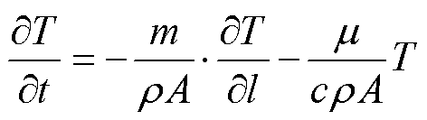 (12)
(12)
热网动态能流方程简化成
 (13)
(13)
 (14)
(14)
热网模型还包括节点的热平衡约束和热损耗约束。
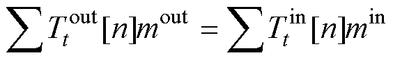
1)热平衡约束
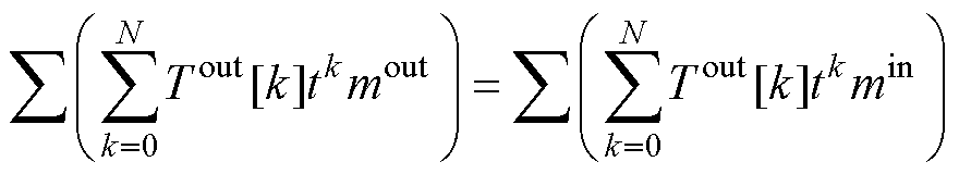
根据能量守恒原理,若假设节点处的热量无损耗,则流入该节点的热能和应该等于流出该节点的热能和,热平衡约束的方程为
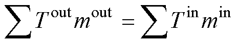 (15)
(15)
式中, 、
、 分别为流入该节点和流出该节点的质量流量。
2)热损耗约束
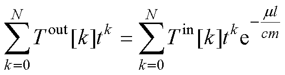
由于热量在传输过程中,外部环境和管道内的水温存在一定温差,导致热水的热量发生损耗,热损耗约束的方程为
 (16)
(16)
全纯嵌入法的核心思想是将一个问题或系统嵌入到一个更简单的域中。本节以时间为变量的全纯函数代替电压幅值、相位和节点温度,重构IHES能流方程。
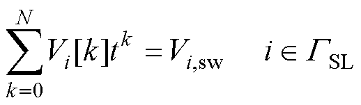
本文用含时间t的全纯函数 描述热网中的节点温度,管道流入、流出温度由幂级数表示为
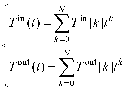 (17)
(17)
式中, 、
、 为管道的首、末端温度幂级数展开的常数项。
则热网偏微分方程组中温度对时间的微分项改写为
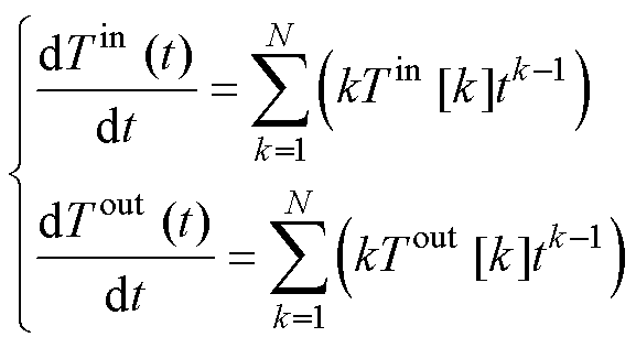 (18)
(18)
将式(17)、式(18)代入式(13)~式(16)中,形成全纯嵌入形式的热网动态能流方程组为
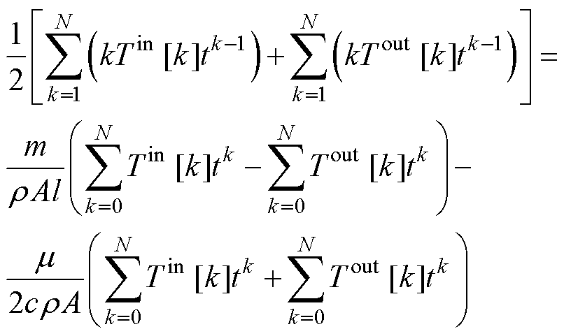 (19)
(19)
 (20)
(20)
 (21)
(21)
 (22)
(22)
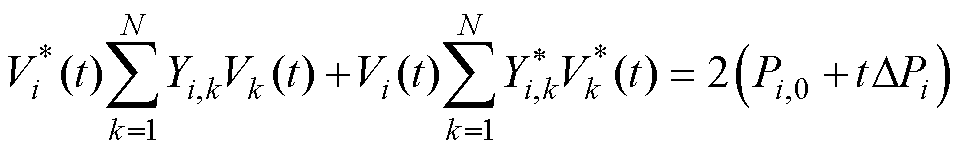
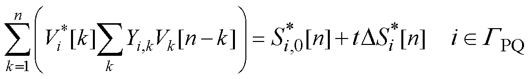
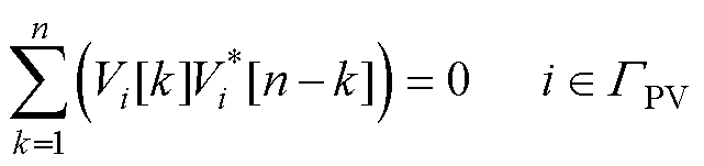
用含时间t的全纯函数 表示节点电压,则式(4)改写为
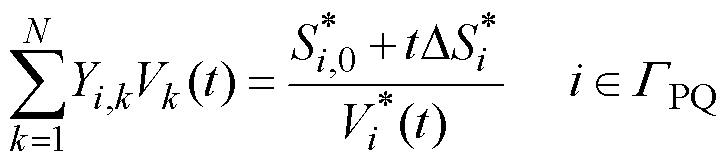 (23)
(23)
 (24)
(24)
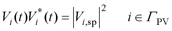 (25)
(25)
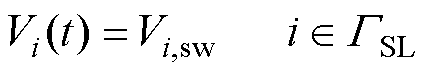 (26)
(26)
式中, 和
和 为参考状态和目标状态下节点的复功率共轭值;
 为节点处目标状态复功率相对参考状态复功率变化量的共轭值;
 和
和 为参考状态和目标状态下节点的注入有功功率;
 为节点处目标状态相对参考状态的有功功率变化量;
 为松弛节点的电压。
对式(23)两边同时乘以 ,将电压同样用幂级数
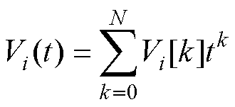 表示,代入式(23)~式(26)中,得到
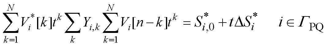 (27)
(27)
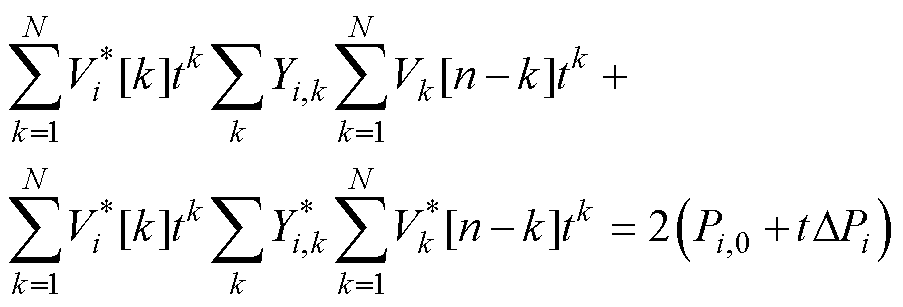
(28)
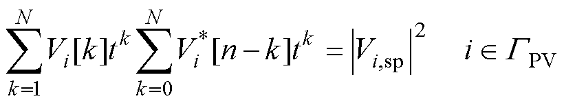 (29)
(29)
 (30)
(30)
用含时间 的全纯函数表示热锅炉机组发出的热功率
 ,以及CHP机组发出的电功率和热功率
 ,并将其全部展开为幂级数形式,则全纯嵌入重构后的电热耦合模型为
 (31)
(31)
 (32)
(32)
所构造的全纯嵌入动态方程满足以下准则:当 时,式(19)~式(22)和式(27)~式(32)为初始参考状态下的全纯嵌入方程组。此时,电力系统与热力系统无耦合,电力系统中负荷母线的电压初值为1.0(pu),而所有母线的相位初值为0°,对于发电机母线(PV母线),电压幅值初值为其额定幅值,而相位依然为0°。而由于IHES中热网的状态量相较于电网的状态量数值波动范围更广,所以其初始变量的猜测较难确定。为了更合理地选取初值,本文选取Newton-Raphson(NR)迭代3次后的稳态能流解作为计算初始点[20]。
由第3节重构的IHES能流方程两侧同阶幂级数系数相等,得到幂级数系数的递归公式。将递归公式展开,提取方程中所有的 项组成新的方程组,得到仅含有n阶幂级数系数的线性方程组,可分别推导热力系统、电力系统及耦合节点递归关系式。
(1)由式(19)~式(22)推导得到热力系统递归关系式为
 (33)
(33)
 (34)
(34)
 (35)
(35)
 (36)
(36)
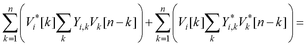
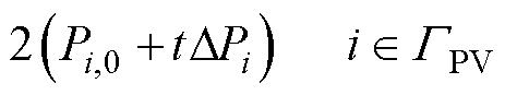
(2)由式(27)~式(30)推导得到电力系统递归关系式为
 (37)
(37)
 (38)
(38)
 (39)
(39)
 (40)
(40)
(3)由式(31)、式(32)推导得到耦合节点递归关系式为
 (41)
(41)
 (42)
(42)
从计算 、
、 和
和 开始,递归求解的过程如下:
(1)已知 、
、 和
和 ,通过比较与同阶项的系数,得到了一组包含高阶系数和低阶系数的线性方程组。
(2)通过求解式(33)~式(42)来计算幂级数的系数、和。
(3)同样求解线性方程组计算得出全纯多项式中的 的系数。
的系数。
因此,全纯多项式中的未知系数在下面的递归范式(43)~式(45)中逐级求解。
 (43)
(43)
 (44)
(44)
 (45)
(45)
从常数项开始,逐阶确定全纯函数幂级数的系数,直到IHES中电力和热能的供应与需求平衡,确定此时的展开阶数[n],代入 到对应阶段的全纯函数
 、
、 和
和 中,可以得到温度和电压的数值解。
全纯嵌入联合动态能流计算具体过程如图4所示,具体步骤如下:
(1) 初始化:选取仿真步长 ,计当前时刻为
 ,即第i阶段的起始时刻;令嵌入变量
 。
。
(2)计算系统状态数据:时刻,代入嵌入变量 ,计算IHES的能流数据,确定全纯函数幂级数展开阶数(展开阶数不大于设定的最大展开阶数,即
 ),并代入全纯方程组,得到代表IHES能流的全纯函数。
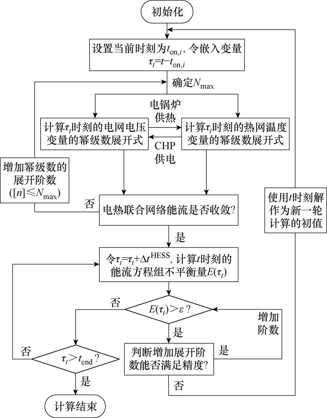
图4 全纯嵌入后的计算流程
Fig.4 The calculation process after holomorphic embedding
(3)计算能流的不平衡量:令 ,并将代入步骤(2),获取新的全纯函数,以计算出系统状态变量的估计值。然后将这些估计值代入电热综合能源系统的微分方程组中,根据式(12)~式(16)计算能流方程组的不平衡量
 。
。
(4)检测不平衡量是否超出标准:计算出的不平衡量若不满足要求,要先增加幂级数的展开阶数,若还是不能满足精度要求则返回到步骤(2)中,将此刻的设为初始值重新计算;若满足要求,则要返回步骤(3)中,令继续计算,直到仿真结束。
本节首先在单热网管道测试案例中验证分析所提HEM的有效性,进一步在IHES算例系统中进行负荷或出力波动仿真分析,验证HESS动态分析的能力。将本文所提方法与龙格库塔法(使用固定时间步长的龙格-库塔法Matlab ODE求解器求解IHES能流方程,下面简称ODE)进行对比。HESS和ODE中的各系数项均通过离线计算给定,仿真时长仅包含在线计算部分,共300 min。选取电力系统的仿真时间步长为0.1 min,热力系统差分时间步长为1 min, =
= =0.5 min,
 ,环境温度
,环境温度 设为20℃。所有仿真在CPU为Intel i9-12900H、内存为8 GB的PC完成,开发环境为Matlab。
本节以单个热网管道为例,对所提的HESS进行仿真验证。热网单管中包含一个热源节点和一个负载节点,由一条9 km的管道连接,其示意图如图5所示,质量流量m=2 500 kg/s,管道直径为1.4 m,横截面面积S=1.54 m2,传热系数 =0.35 W/(m·K)[17]。
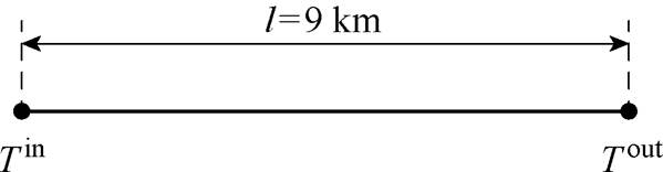
图5 单热网管道算例示意图
Fig.5 Schematic diagram of single heat-supply network pipeline
在整个仿真期间设置一种运行场景进行测试:在系统稳定运行(供应或需求没有变化)30 min后,将热源温度在60 min内提高到100℃。按照4.2节中的全纯嵌入IHES能流计算方案,得到IHES能流的解析解。
以t=30 min时的末端温度为例,开始一个新的阶段,此时 =30 min,
 为该阶段的嵌入量,
 ,
, ,则末端温度全纯函数为
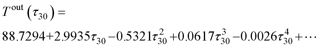 (46)
(46)
在t=31 min时, ,代入式(46),可计算出此时刻的末端温度。HESS重复4.2节的计算步骤计算出每个阶段的全纯函数,进而得到整个仿真期间的末端温度如图6所示。
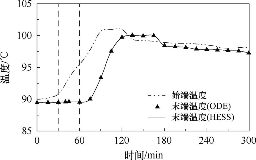
图6 算例1仿真结果
Fig.6 Example 1 simulation results
HESS的仿真结果是由若干个如式(46)所示的全纯函数连接而成,每一个全纯函数代表一个时间段,在时间段内任意时间断面的能流解都可以通过将代入该阶段全纯函数进行计算,即可做到直接求解任意时刻的IHES的工作状态。而ODE只能通过不断的迭代获取时间断面下的能流解,所以将ODE的仿真结果用散点图来表示。
将HESS仿真结果与ODE的计算结果进行比较,两种结果几乎相等。这表明,所提出的HESS方法可以得到与其他常用求解方法类似的计算结果。从图6中曲线可以观察到,末端温度与始端温度的变化趋势几乎相同。由于热网的传输时延特性,末端温度的曲线相较于始端温度向右发生了偏移。同时由于热网管道的动态特性,管道内的温度传输会发生损耗,所以末端温度较始端温度有所 下降。
全纯嵌入法和龙格库塔定步长算法对比如图7所示,由于ODE需要在定步长 的前提下,不断地迭代,求得离散时间下的能流解(在仿真结果中用散点图的形式来表达)。要想获得时间段中的系统状态变量,需要重新求解,这会导致计算效率大大降低,且其保证精度的方法是选取足够小的,而HESS可以输出连续的能流解,只需递归求解一遍(仅当不平衡量
 不满足要求时,才需要重新计算全纯函数),即可得到能流关于时间的显示表达式,无需重复迭代求解。
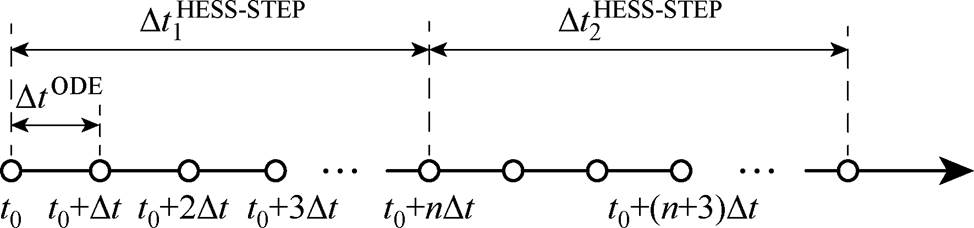
图7 全纯嵌入法和龙格库塔定步长算法对比
Fig.7 Comparison between holomorphic embedding method and Runge-Kutta step-size algorithm
5.2.1 算例介绍
本节对所提的HESS进行测试分析。利用51节点热力网络和IEEE 14节点的电力网络标准算例耦合成的电热综合能源系统进行分析计算[15],热力网络线路的具体数据见附录,系统拓扑结构如图8所示。CHP为燃气轮机,连接电网的节点14和热网的节点1,工作在以热定电的模式下,是热网的主供热源;电锅炉机组连接热网的节点14和电网的节点1,是热网的次供热源,电锅炉的效率通常在90%~98%之间,本文将电锅炉效率设为90%。
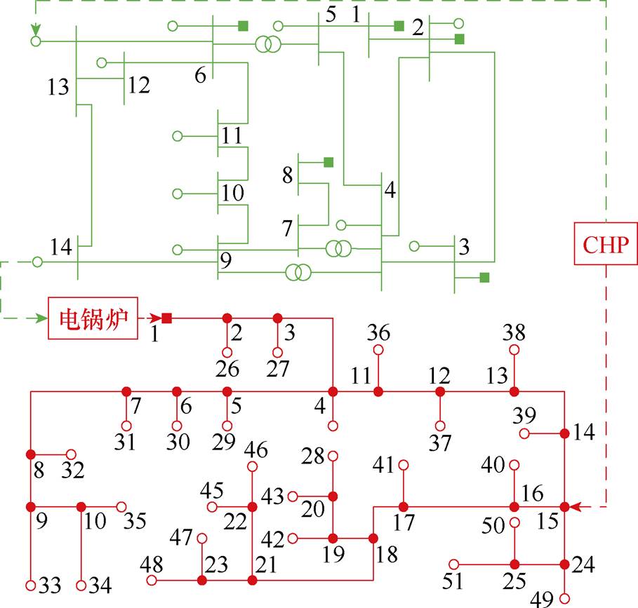
图8 IHES算例拓扑
Fig.8 IHES example topology
5.2.2 负荷和出力波动场景划分
为了展示本文所提的HESS连续时间分析和响应波动的能力,设置以下三种方案进行运行测试,给出了动态仿真的结果,并将HESS计算结果与文献[19]提出的HEFS、文献[20]提出的FFHE及传统的ODE所得的能流解进行比较:
场景1:热网中节点37处的热负荷逐渐增加(在150 min内增加至原来的110%)。
场景2:电网中节点4处负荷增加(瞬间上升20%),热网中节点46处热负荷逐渐增加(在150 min内增加至原来的105%)。
场景3:电网中节点1处发电机出力增加(90 s内上升10 MW),热网中温度也随之发生变化。
设置电网、热网方程的不平衡量标准分别为 和
和 。已知发生扰动之前此IHES已稳定运行了60 min。
5.2.3 仿真结果分析
算例2中的场景1~场景3仿真结果如图9~图11所示。HEFS将IHES拆分成电力系统和热力系统分别进行计算,导致在热网发生波动的情况下,负荷节点的温度无法及时响应工况的变化,所得的动态能流解存在误差;FFHE利用灵活快速的全纯嵌入,重构综合能源系统稳态模型,计算结果为波动后恢复稳态的某一时间断面下的能流解,即其仿真结果在图9~图11中表示为一个点。
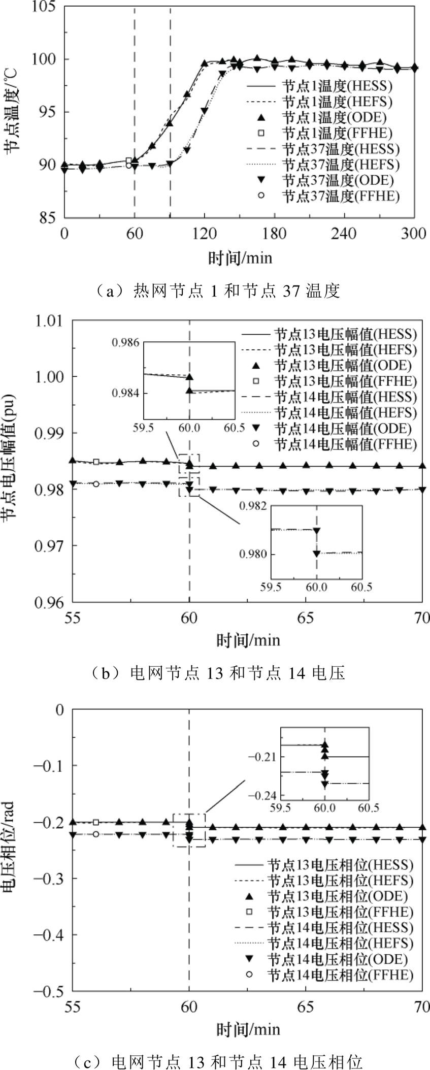
图9 算例2场景1仿真结果
Fig.9 Simulation results of scenario 1 in example 2
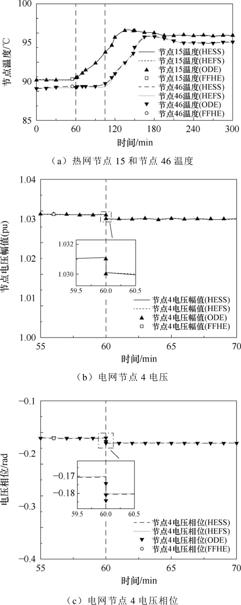
图10 算例2场景2仿真结果
Fig.10 Simulation results of example 2 in scenario 2
场景1:如图9b和图9c所示,热网的节点37负荷增加,电锅炉和CHP需增加出力满足负荷需求,导致电网中线路损耗和压降增大,使电力网络中的负荷节点13和节点14电压幅值和相位下降。同时,如图9a所示,因为热锅炉连接热力系统节点1,节点1的温度迅速增加,节点37由于距离热源节点较远,延迟约31 min后开始增加。
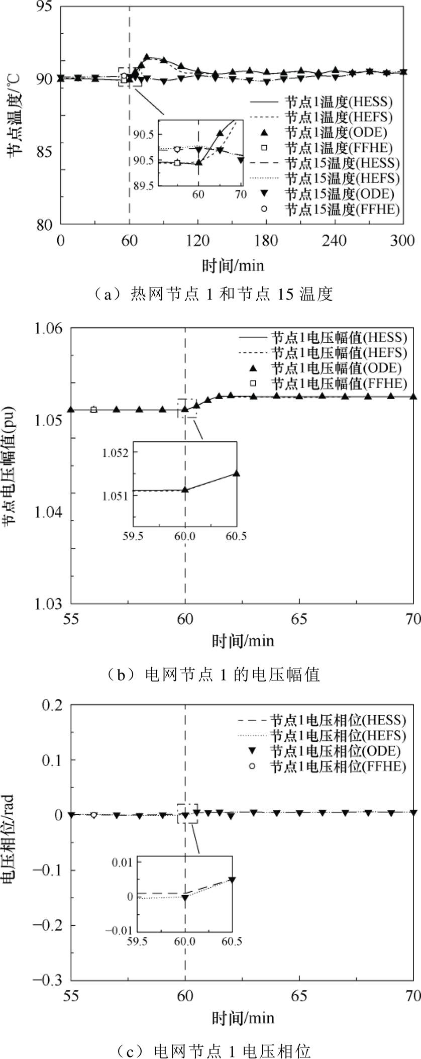
图11 算例2场景3仿真结果
Fig.11 Simulation results of example 2 in scenario 3
场景2:如图10a所示,热网的节点46温度增加的同时,电网中节点4的负荷瞬时增加,导致电力系统发电机和CHP自动增加出力。热网节点15由于直接与CHP相连,在CHP出力增加的同时,温度逐渐上升,而节点46属于热负荷的末端节点,与热源节点的实际空间距离较远,其温度延迟约46.5 min后开始逐渐增加。如图10b和图10c所示,节点4负荷增加导致更大的电压降,电力系统中传输的有功无功增加,导致节点4的电压和相位降低。
场景3:如图11a所示,电网中节点1发电机出力增加,导致热网中与电网直接相连的节点1温度立刻上升,而CHP工作在以热定电的模式下,所以与其相连的节点15温度没有明显变化,整个热网温度在5 min后趋于稳定。如图11b和11c所示,发电机出力增加,导致有功无功增加,发电机节点电压相位发生略微上升。
三个场景下HESS、HEFS、ODE和FFHE的计算时间,见表1。三个场景下HESS、HEFS、FFHE与ODE的计算结果的最大相对误差,见表2。HESS在计算全纯函数幂级数展开式的过程中,只需判断一次IHES能流是否收敛,无需反复判断子系统能流是否收敛,这大大节省了计算时间;HEFS需要对子系统不断地进行重复迭代,导致计算时间较长;传统的ODE需要选取较小的来保证计算精度,这大大延长了计算速度;而FFHE通过稳态方程建模,只计算某个时间断面下的能流解,拥有较好的计算速度和精度。
表1 算例2计算时间对比
Tab.1 Example 2 calculation time comparison (单位: s)
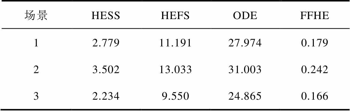
场景HESSHEFSODEFFHE 12.77911.19127.9740.179 23.50213.03331.0030.242 32.2349.55024.8650.166
表2 算例2计算结果最大相对误差
Tab.2 Example 2 calculates the maximum relative error of the result

求解算法场景最大相对误差(%) 节点温度电压幅值电压相位 ODE1——— 2 3 HESS11.982 7×10-52.835 2×10-73.124 7×10⁻⁸ 28.070 1×10-63. 775 7×10-72.317 4×10⁻⁸ 35.053 3×10-63.570 4×10-78.150 6×10⁻⁷ HEFS13.089 9×10-48.214 5×10-67.374 1×10⁻⁶ 28.410 1×10-31.013 3×10-57.001 3×10⁻⁶ 37.748 2×10-59.118 5×10-67.809 5×10⁻⁶ FFHE15.975 7×10-72.070 3×10-84.008 4×10⁻⁸ 24.342 8×10-71.690 5×10-89.345 9×10⁻⁹ 37.083 7×10-72.612 5×10-86.723 4×10⁻⁸
本文提出了一种基于全纯嵌入的IHES动态能流计算方法。该方法将热网偏微分方程和电网潮流方程重构,并利用全纯嵌入联合求解法,递归计算得到IHES的动态能流解析解,最后通过仿真算例分析验证了方法的有效性。主要结论如下:
1)所提能流计算方法利用全纯函数可直接计算仿真时间内任意时刻的电热综合能源系统的工作状态。相比于全纯嵌入分解求解法和传统的龙格库塔法,本文所提方法更加灵活且高效。
2)所提能流计算方法可用于电热综合能源系统的动态仿真,特别是在负荷或出力发生波动的情况下,可以连续地分析系统的运行状态并精准地描述能流响应扰动的过程。
需要指出的是,本文所提的动态能流计算方法未考虑新能源出力和负荷的不确定性,拟在后续研究中进一步考虑。
附 录
附表1 51节点热网节点数据
App.Tab.1 Data of 51-node heat supply network nodes

节点编号节点类型质量流量/ (kg/s)节点编号节点类型质量流量/ (kg/s) 10-302.2227110 21028110 31029111.11 41030111.11 51031111.11 61032111.11 71033111.11 81034111.11 91035111.11 101036110 111037110 121038113.33 131039113.33 141040113.33 151041111.11 161042111.11 171043111.11 181044111.11 191045111.11 201046111.11 211047111.11 221048111.11 231049114.46 241050114.46 251051114.46 26110———
注:节点类型中,热源节点为0,其他节点为1。
附表2 51节点热网线路数据
App.Tab.2 Line data of 51-node heat supply network
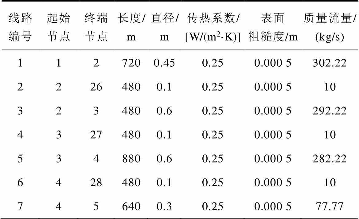
线路编号起始节点终端节点长度/ m直径/ m传热系数/ [W/(m2·K)]表面粗糙度/m质量流量/ (kg/s) 1127200.450.250.000 5302.22 22264800.10.250.000 510 3234800.60.250.000 5292.22 43274800.10.250.000 510 5348800.60.250.000 5282.22 64284800.10.250.000 510 7456400.30.250.000 577.77
注:节点类型中,热源节点为0,其他节点为1。
(续)
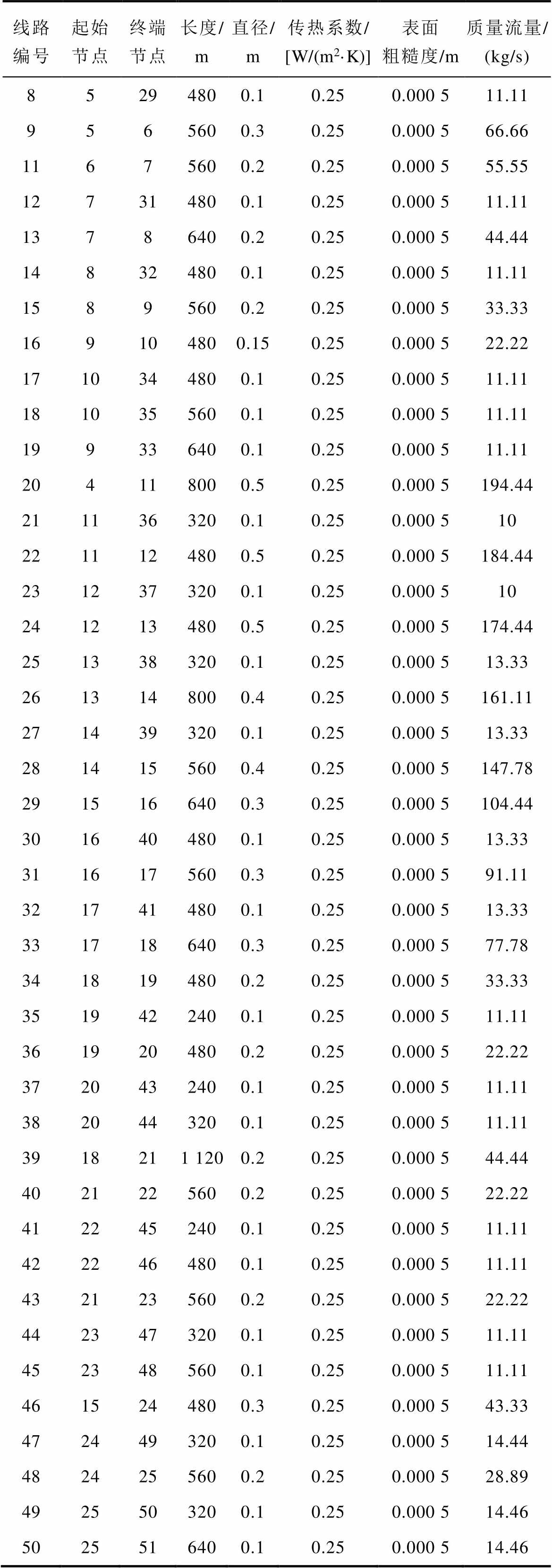
线路编号起始节点终端节点长度/ m直径/ m传热系数/ [W/(m2·K)]表面粗糙度/m质量流量/ (kg/s) 85294800.10.250.000 511.11 9565600.30.250.000 566.66 11675600.20.250.000 555.55 127314800.10.250.000 511.11 13786400.20.250.000 544.44 148324800.10.250.000 511.11 15895600.20.250.000 533.33 169104800.150.250.000 522.22 1710344800.10.250.000 511.11 1810355600.10.250.000 511.11 199336400.10.250.000 511.11 204118000.50.250.000 5194.44 2111363200.10.250.000 510 2211124800.50.250.000 5184.44 2312373200.10.250.000 510 2412134800.50.250.000 5174.44 2513383200.10.250.000 513.33 2613148000.40.250.000 5161.11 2714393200.10.250.000 513.33 2814155600.40.250.000 5147.78 2915166400.30.250.000 5104.44 3016404800.10.250.000 513.33 3116175600.30.250.000 591.11 3217414800.10.250.000 513.33 3317186400.30.250.000 577.78 3418194800.20.250.000 533.33 3519422400.10.250.000 511.11 3619204800.20.250.000 522.22 3720432400.10.250.000 511.11 3820443200.10.250.000 511.11 3918211 1200.20.250.000 544.44 4021225600.20.250.000 522.22 4122452400.10.250.000 511.11 4222464800.10.250.000 511.11 4321235600.20.250.000 522.22 4423473200.10.250.000 511.11 4523485600.10.250.000 511.11 4615244800.30.250.000 543.33 4724493200.10.250.000 514.44 4824255600.20.250.000 528.89 4925503200.10.250.000 514.46 5025516400.10.250.000 514.46
参考文献
[1] 胡枭, 尚策, 程浩忠, 等. 综合能源系统能流计算方法述评与展望[J]. 电力系统自动化, 2020, 44(18): 179-191.
Hu Xiao, Shang Ce, Cheng Haozhong, et al. Review and prospect of calculation method for energy flow in integrated energy system[J]. Automation of Electric Power Systems, 2020, 44(18): 179-191.
[2] 亢猛, 钟祎勍, 石鑫, 等. 计及负荷供给可靠性的园区综合能源系统两阶段优化方法研究[J]. 发电技术, 2023, 44(1): 25-35.
Kang Meng, Zhong Yiqing, Shi Xin, et al. Research on two-stage optimization approach of community integrated energy system considering load supply reliability[J]. Power Generation Technology, 2023, 44(1): 25-35.
[3] Martinez-Mares A, Fuerte-Esquivel C R. A unified gas and power flow analysis in natural gas and electricity coupled networks[J]. IEEE Transactions on Power Systems, 2012, 27(4): 2156-2166.
[4] 孙国强, 王文学, 吴奕, 等. 辐射型电-热互联综合能源系统快速潮流计算方法[J]. 中国电机工程学报, 2020, 40(13): 4131-4142.
Sun Guoqiang, Wang Wenxue, Wu Yi, et al. Fast power flow calculation method for radiant electric- thermal interconnected integrated energy system[J]. Proceedings of the CSEE, 2020, 40(13): 4131-4142.
[5] 赵霞, 王骆, 谭红, 等. 适用于压缩机定速控制的电-气综合能流计算方法[J]. 电力系统自动化, 2022, 46(21): 116-124.
Zhao Xia, Wang Luo, Tan Hong, et al. Calculation method of integrated electricity-gas energy flow for compressors with constant speed control[J]. Auto- mation of Electric Power Systems, 2022, 46(21): 116-124.
[6] 刘鹏飞, 武家辉, 王海云, 等. 计及氢气注入与压缩因子的综合能源系统能流计算[J]. 电力系统保护与控制, 2024, 52(2): 118-128.
Liu Pengfei, Wu Jiahui, Wang Haiyun, et al. Calculation of energy flow in integrated energy systems with hydrogen injection and compression factors[J]. Power System Protection and Control,
2024, 52(2): 118-128.
[7] 钟俊杰, 李勇, 曾子龙, 等. 综合能源系统多能流准稳态分析与计算[J]. 电力自动化设备, 2019, 39(8): 22-30.
Zhong Junjie, Li Yong, Zeng Zilong, et al. Quasi- steady-state analysis and calculation of multi-energy flow for integrated energy system[J]. Electric Power Automation Equipment, 2019, 39(8): 22-30.
[8] 苏洁莹, 林楷东, 张勇军, 等. 基于统一潮流建模及灵敏度分析的电-气网络相互作用机理[J]. 电力系统自动化, 2020, 44(2): 43-52.
Su Jieying, Lin Kaidong, Zhang Yongjun, et al. Interaction mechanism of electricity-gas network based on unified power flow modeling and sensitivity analysis[J]. Automation of Electric Power Systems, 2020, 44(2): 43-52.
[9] Gu Wei, Wang Jun, Lu Shuai, et al. Optimal operation for integrated energy system considering thermal inertia of district heating network and buildings[J]. Applied Energy, 2017, 199: 234-246.
[10] Stevanovic V D, Zivkovic B, Prica S, et al. Prediction of thermal transients in district heating systems[J]. Energy Conversion and Management, 2009, 50(9): 2167-2173.
[11] Wang Yaran, You Shijun, Zhang Huan, et al. Thermal transient prediction of district heating pipeline: Optimal selection of the time and spatial steps for fast and accurate calculation[J]. Applied Energy, 2017, 206: 900-910.
[12] Yao Shuai, Gu Wei, Lu Shuai, et al. Dynamic optimal energy flow in the heat and electricity integrated energy system[J]. IEEE Transactions on Sustainable Energy, 2021, 12(1): 179-190.
[13] 杨经纬, 张宁, 康重庆. 多能源网络的广义电路分析理论: (一)支路模型[J]. 电力系统自动化, 2020, 44(9): 21-32.
Yang Jingwei, Zhang Ning, Kang Chongqing. Analysis theory of generalized electric circuit for multi-energy networks: part one branch model[J]. Automation of Electric Power Systems, 2020, 44(9): 21-32.
[14] 杨经纬, 张宁, 康重庆. 多能源网络的广义电路分析理论: (二)网络模型[J]. 电力系统自动化, 2020, 44(10): 10-21.
Yang Jingwei, Zhang Ning, Kang Chongqing. Analysis theory of generalized electric circuit for multi-energy networks: part two network model[J]. Automation of Electric Power Systems, 2020, 44(10): 10-21.
[15] 陈彬彬, 孙宏斌, 陈瑜玮, 等. 综合能源系统分析的统一能路理论(一): 气路[J]. 中国电机工程学报, 2020, 40(2): 436-444.
Chen Binbin, Sun Hongbin, Chen Yuwei, et al. Energy circuit theory of integrated energy system analysis (Ⅰ): gaseous circuit[J]. Proceedings of the CSEE, 2020, 40(2): 436-444.
[16] 陈彬彬, 孙宏斌, 尹冠雄, 等. 综合能源系统分析的统一能路理论(二): 水路与热路[J]. 中国电机工程学报, 2020, 40(7): 2133-2142, 2393.
Chen Binbin, Sun Hongbin, Yin Guanxiong, et al. Energy circuit theory of integrated energy system analysis(Ⅱ): hydraulic circuit and thermal circuit[J]. Proceedings of the CSEE, 2020, 40(7): 2133-2142, 2393.
[17] 张苏涵, 顾伟, 姚帅, 等. 综合能源网络统一建模及其应用(一): 时域二端口模型[J]. 中国电机工程学报, 2021, 41(19): 6509-6521.
Zhang Suhan, Gu Wei, Yao Shuai, et al. Unified modeling of integrated energy networks in time domain and its applications(Ⅰ): two-port models in time domain[J]. Proceedings of the CSEE, 2021, 41(19): 6509-6521.
[18] Trias A. The holomorphic embedding load flow method[C]//2012 IEEE Power and Energy Society General Meeting, San Diego, CA, USA, 2012: 1-8.
[19] 刘承锡, 徐慎凯, 赖秋频. 基于全纯嵌入法的非迭代电力系统最优潮流计算[J]. 电工技术学报, 2023, 38(11): 2870-2882.
Liu Chengxi, Xu Shenkai, Lai Qiupin. Non-iterative optimal power flow calculation based on holomorphic embedding method[J]. Transactions of China Elec- trotechnical Society, 2023, 38(11): 2870-2882.
[20] Zhang Tong, Li Zhigang, Wu Qiuwei, et al. Dynamic energy flow analysis of integrated gas and electricity systems using the holomorphic embedding method[J]. Applied Energy, 2022, 309: 118345.
[21] Ma Houzhen, Liu Chunyang, Zhao Haoran, et al. A novel analytical unified energy flow calculation method for integrated energy systems based on holomorphic embedding[J]. Applied Energy, 2023, 344: 121163.
[22] 潘超, 范宫博, 王锦鹏, 等. 灵活性资源参与的电热综合能源系统低碳优化[J]. 电工技术学报, 2023, 38(6): 1633-1647.
Pan Chao, Fan Gongbo, Wang Jinpeng, et al. Low-carbon optimization of electric and heating integrated energy system with flexible resource participation[J]. Transactions of China Electro- technical Society, 2023, 38(6): 1633-1647.
[23] 张义志, 王小君, 和敬涵, 等. 考虑供热系统建模的综合能源系统最优能流计算方法[J]. 电工技术学报, 2019, 34(3): 562-570.
Zhang Yizhi, Wang Xiaojun, He Jinghan, et al. Optimal energy flow calculation method of integrated energy system considering thermal system modeling[J]. Transactions of China Electrotechnical Society, 2019, 34(3): 562-570.
[24] 朱浩昊, 朱继忠, 李盛林, 等. 基于Benders分解和纳什议价的分布式热电联合优化调度[J]. 电工技术学报, 2023, 38(21): 5808-5820.
Zhu Haohao, Zhu Jizhong, Li Shenglin, et al. Distributed combined heat and power optimal scheduling based on Benders decomposition and Nash bargaining[J]. Transactions of China Electrotechnical Society, 2023, 38(21): 5808-5820.
[25] 梁炜焜, 林舜江, 刘明波, 等. 基于供冷/热系统质-量调节的区域综合能源系统动态最优能流计算[J].电网技术, 2024, 48(3): 1008-1021.
Liang Weikun, Lin Shunjiang, Liu Mingbo, et al. Dynamic optimal energy flow calculation of regional integrated energy system based on quality-quantity regulation of cooling/heating system[J]. Power System Technology, 2024, 48(3): 1008-1021.
Abstract Integrated energy system (IES) is a product of the deep integration between multiple energy networks and the internet. It aims to enhance the comprehensive utilization of various forms of energy, such as electricity, heat, cooling, and gas, by establishing supply, transmission, distribution, and utilization systems. The dynamic simulation calculations of the IES are crucial for subsequent optimization control and energy scheduling research. This paper proposes a dynamic energy flow calculation method for the integrated heat and electricity systems (IHES) based on holomorphic embedding to accurately describe the dynamic characteristics of thermal network pipelines and achieve continuous dynamic simulation of the IHES.
Firstly, the study spatially discretizes the dynamic model of thermal network pipelines in the IHES, keeping the differential relationship of temperature concerning time, and the partial differential equation of heat network is transformed into an ordinary differential equation. A thermal network model under mass regulation mode is proposed. Secondly, the energy flow equation is reconstructed with a time-varying holomorphic function, and the dynamic electric-thermal energy flow model is established by holomorphic embedding. Then, using the holomorphic embedding sequence solution (HESS) method to determine the series unfolding sequence, the analytical expressions of node temperature, voltage amplitude, and phase with time can be obtained. Finally, a single thermal pipeline serves as a case study to compare the HESS with the Runge-Kutta method. Simulation results indicate that the HESS can produce a continuous energy flow solution with one recursive calculation (recalculation of holomorphic functions is only necessary when imbalances do not meet the requirements). By inserting time into the current phase of holomorphic functions, the IHES state variable values can be determined without repetitive iterative solutions. In contrast, the Runge-Kutta method requires continuous iteration with a fixed step size to obtain discrete-time energy flow solutions, and its accuracy assurance method involves choosing sufficiently small step sizes, leading to longer computational times.
Simulation analysis is conducted on an IEEE 14-node standard case and a 51-node thermal network. By setting scenarios of increased thermal load, simultaneous increase in electrical and thermal loads, and increased generator output, the simulation results are compared with the holomorphic embedding factorization solution (HEFS), fast and flexible holomorphic embedding (FFHE), and Runge-Kutta method. HEFS requires continuous repetitive iterations on subsystems, resulting in longer computation times and lower precision. FFHE, however, models steady-state equations to calculate energy flow solutions at specific time slices, offering better computational speed and precision.
The following conclusions are drawn from the simulation analysis. (1) HESS utilizes holomorphic functions to directly calculate the working state of IHES at any moment within the simulation time. The proposed method is more flexible and efficient than the holomorphic embedding decomposition and traditional Runge-Kutta methods. (2) The proposed energy flow calculation method can be used for dynamic simulation of electric- thermal integrated energy systems, especially in load or output fluctuation cases, to continuously analyze the system’s operational state and accurately describe the energy flow process response to disturbances.
keywords:Holomorphic embedding method, energy flow calculation, dynamic simulation, recursive computation
DOI: 10.19595/j.cnki.1000-6753.tces.240196
中图分类号:TM743
收稿日期 2024-01-29
改稿日期 2024-04-10
李宏仲 男,1977年生,副教授,研究方向为综合能源系统规划、配电网承载能力评估等。E-mail: lhz_ab@263.net
滕佳伦 男,1999年生,硕士研究生,研究方向为综合能源系统优化。E-mail: tengjia7un@163.com(通信作者)
(编辑 陈 诚)