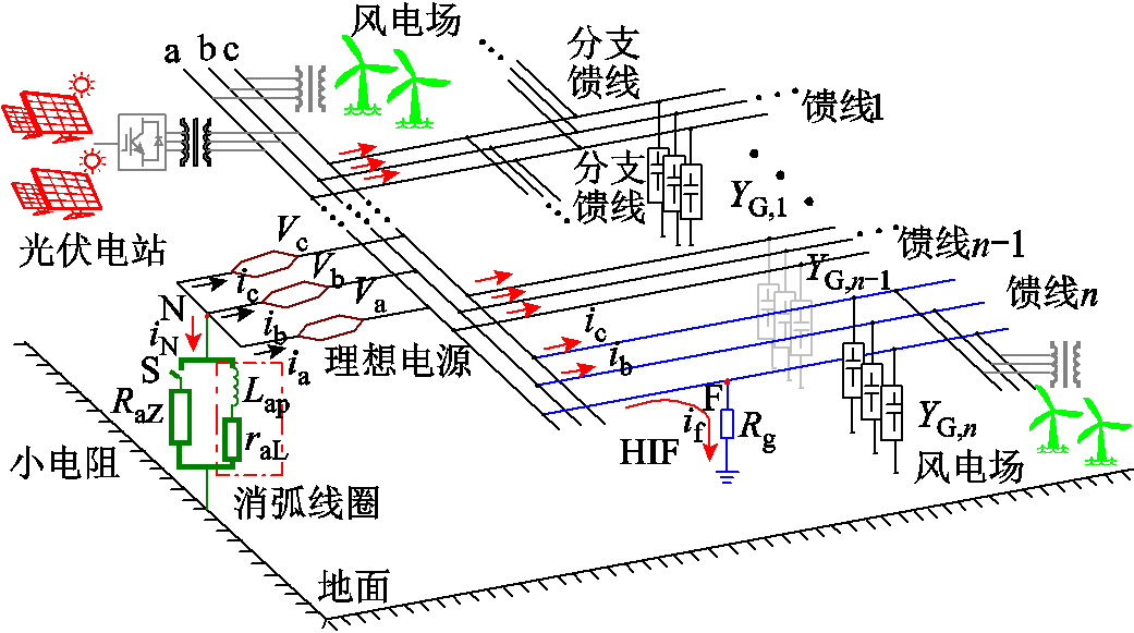
图1 灵活接地配电系统示意图
Fig.1 Flexible grounding distribution systems
摘要 针对灵活接地配电系统在发生高阻故障时,无法实现准确选线的问题,通过分析灵活接地系统故障特征得出中性点小电阻投入后故障馈线与健全馈线在零序电流幅值上存在差异,同时,小电阻投入后母线零序电压发生明显降低。由此,提出一种基于中性点小电阻投入前后不同时段下计算内积投影的高阻故障选线方法。首先,将小电阻投入后各馈线零序电流对投入前的母线零序电压做内积投影,由此构建判据1;其次,将小电阻投入后各馈线零序电流对投入前的中性点电流做内积投影,由此构建判据2;最后,当判据1与判据2判定的故障馈线结果一致时,得到故障馈线。大量仿真实验表明,在非同步采样、数据缺失与电弧等故障工况下,该方法具有良好的稳定性,与现有方法对比可知,该文方法判定时间短,且适应电流互感器反接工况。
关键词:灵活接地系统 高阻故障 不同时段 内积投影
高阻故障是一种常见的配电网故障形式,约占中压配电网故障的5%~20%,故障特征弱。对于阻抗非常高的一些接地材料,电流幅值仅有数安培,传统保护无法保证可靠性。如果不能及时检测出故障馈线,可能会导致大规模停电或森林火灾,且存在人身触电的风险[1]。因此,研究高阻故障选线技术具有重要意义。
近些年,国内外学者对高阻故障选线进行了大量研究,可将现有技术分为被动式[1-9]与主动式[10-11]两类。
1)被动式。文献[1]提出了同步3次谐波的群体比相选线法,但该方法在互感器反接、异步采样等极端工况中可能存在误判。文献[2]利用内积原理构造综合内积值,通过幅值与相位判据实现高阻故障选线。文献[3]依据消弧线圈补偿特性反映的电流份额变化构造选线判据,该方法可以适应复杂工况,但当配电网结构发生变化时,判据中的阈值可能需要调整。文献[4]使用特定频带的伏安特性轨迹检测故障馈线,但该方法的准确性受限于互感器极性。文献[5]利用故障馈线与健全馈线投影系数的差异实现高阻故障选线。文献[6]将互补集合经验模态分解应用于故障检测。文献[7]使用基频分量移位法提取精准的暂态信号,通过拉普拉斯分布将暂态能量和余弦相似度相结合构造最终选线判据。文献[8]利用S变换提取各馈线时频域行波全景波形,分析全景波形中幅值、频率和极性的差异性,构造综合相关系数区分故障线路和健全线路,但该方法在复杂工况下的适应性有待分析。文献[9]借助模糊C均值聚类算法实现故障馈线检测,但该方法在实际应用中检测时间较长。
2)主动式。文献[10]提出一种有源逆变器与小电阻结合的接地方式,可以提高故障处理能力,但变压器接地方式改动较大。文献[11]在中性点注入电流增量,比较线路电流变化量与电压变化量之间的关系实现选线,但注入电流增量大小需随着配电网结构变化。文献[12]首先获得消弧线圈调节后的馈线电流轨迹,再结合灰色关联度识别故障馈线。文献[13]在消弧线圈调节的基础上构造了基于电流空间相对距离的故障选线技术。除此以外,基于灵活接地系统的主动式在高阻故障选线中具有较好应用前景[14-21],该系统兼顾了谐振接地系统与小电阻接地系统优点,同时可以实现熄灭电弧与故障馈线检测。文献[14]系统分析了传统保护在灵活接地系统中的适应性,得出传统保护无法识别并联小电阻是否投入,且会进一步导致保护性能下降的结论。文献[15]为减少小电阻投入次数提出了一种故障检测策略。文献[16]分析了小电阻投入前后负序电压的变化量,并结合零序电流在负序方向的投影,进而判断出故障分支,但该方法原理复杂。文献[17]在小电阻投入前使用零序电流能量判断故障馈线,小电阻投入后使用零序电流与母线电压相位差实现选线,但该方法在异步采样工况中可能会误判。文献[18]使用并联小电阻投入前后零序测量导纳特征实现故障选线,检测的准确性与互感器极性、互感器精度有关。文献[19]基于小电阻投入前后馈线电流与中性点电流的相位构造选线判据。文献[20-21]基于小电阻投入前后馈线电流与母线电压相位构造高阻故障选线判据。
通过分析发现,现有方法存在以下两个问题:
1)现有高阻故障选线方法原理复杂,计算过程繁琐,同时现有灵活接地系统判据在构造时使用了小电阻投入后母线电压,但是高阻故障时小电阻投入会使母线电压明显减小,因此,仅采用小电阻投入后同一时间尺度内电流与电压进行判据构建时,检测准确性易受影响。
2)现有的高阻故障选线方法大多采用单一判据,无法适应多变的故障工况,因此,存在适应性较弱的问题,特别是在极端故障工况下可靠性无法保证。
针对现有方法存在的问题,本文分析了灵活接地系统故障特征及不同时段下内积投影,提出基于不同时段内积投影的灵活接地系统高阻故障选线方法。将小电阻投入后各馈线零序电流对小电阻投入前母线零序电压和中性点零序电流计算内积投影值,充分利用不同时段下的故障特征,进一步简化了选线判据原理,解决了小电阻投入后电压大幅降低带来的问题,并在构建判据时采用互补性原理构建选线判据。大量仿真测试表明,本文方法具有有效性。
图1为10 kV灵活接地配电系统系统示意图,图中,Rg为接地电阻,RaZ为小电阻,Lap为消弧线圈电感,raL为消弧线圈有功损耗电阻,Va、Vb、Vc为三相电源电压,YG为线路导纳。工作原理为:配电网正常运行时,小电阻控制开关S处于断开状态,中性点仅通过消弧线圈接地;当发生瞬时性接地故障时,消弧线圈立即工作,补偿接地电流,实现熄灭电弧并抑制其重燃;若瞬时性故障发展为永久性故障,S闭合,10 Ω小电阻投入[18],作用是抑制故障过电压及实现故障检测。
图1 灵活接地配电系统示意图
Fig.1 Flexible grounding distribution systems
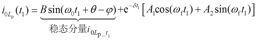
分析可知,当S处于断开状态时,灵活接地系统可等效为谐振接地系统,发生高阻故障时,馈线电感、馈线电阻、raL可以忽略。因此,零序等效网络如图2所示。图中,Lp=3Lap,过补偿度为10%,该系统共有n条馈线,假定第n条馈线为故障馈线,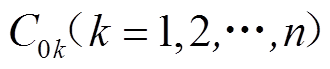 为第k条馈线对地电容,R=3Rg;i0k为第k条馈线的零序电流,i0f与
 分别为故障点零序电流与中性点电流,u0f与u0(t1)分别为故障点零序电压与母线零序电压。
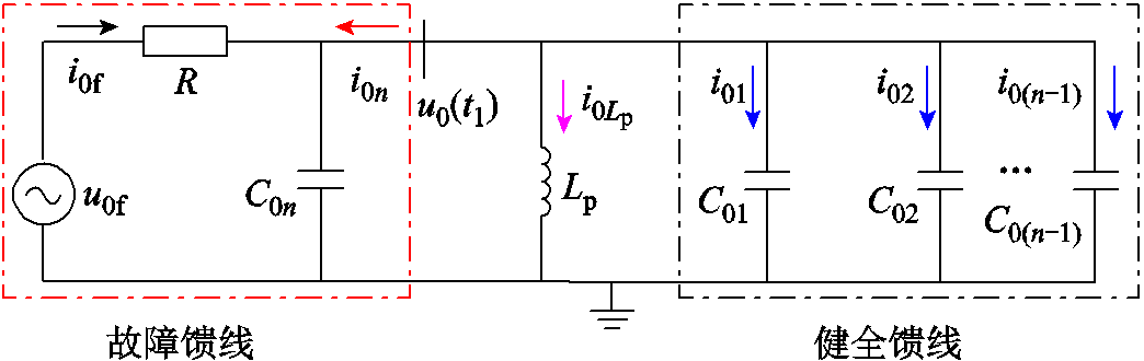
图2 谐振接地系统零序等效网络
Fig.2 Zero sequence network of resonant grounded system
依据图2,列写二阶微分方程为
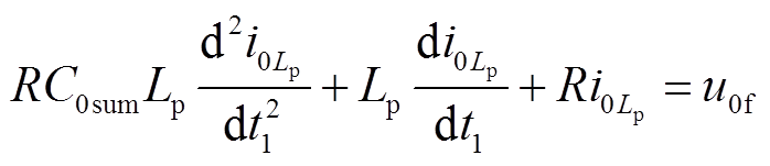 (1)
(1)
式中,C0sum为各馈线对地电容之和,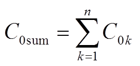 。
。
当满足式(2)时,系统呈现欠阻尼状态。
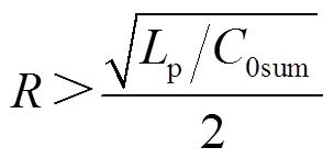 (2)
(2)
定义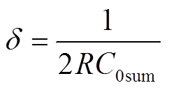 ,
,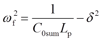 。
。
设u0f =Umsin(ω0t1+θ),Um与θ分别为故障点电压幅值与初相角,ω0为工频角频率。
中性点零序电流为
 (3)
(3)
母线零序电压为
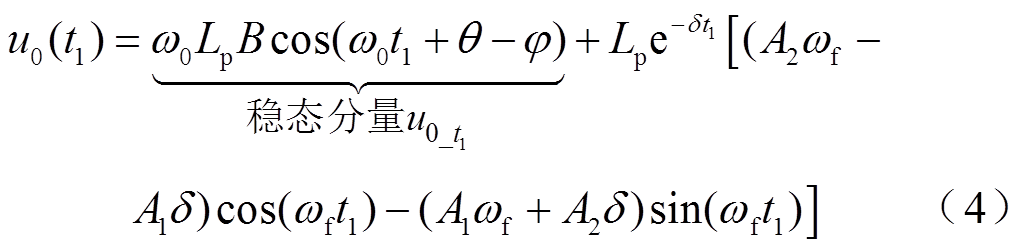
健全馈线零序电流为

式中, 。
。
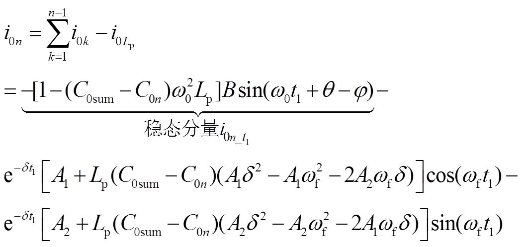
故障馈线零序电流为
 (6)
(6)
其中

由于配电网实际对地电容电流大于10 A时采用谐振接地系统,且对地电容电流一般不大于200 A,因此,设定图2对地电容电流范围在10~200 A[18-20]。C0sum随着对地电容电流的增加而增加,其范围为1.84~36.8 μF,Lp随着对地电容电流的增加而减小,其范围为0.25~5.01 H。根据C0sum与Lp可以求解出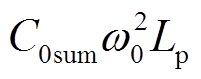 的数值变化如图3所示,其数值小于1,则
 。对比式(5)与式(6)可得,
 与
与 相位一致,不受对地电容电流增加的影响,因此,基于小电阻投入前相位差异的稳态分量检测方法无法实现故障选线。
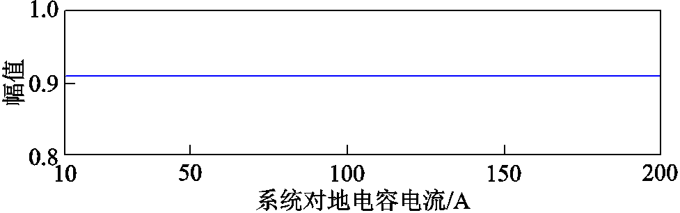
图3 稳态分量幅值
Fig.3 Steady-state component amplitudes
当瞬时性故障发展为永久故障时,开关S闭合,小电阻与消弧线圈并联的等效阻抗由电阻r与电抗ω0L组成。考虑对地电容电流变化范围,可得Lap随着对地电容电流的增加而减小,其范围为0.084~1.67 H,raL随着对地电容电流的增加而减小,其范围为0.66~13.12 Ω。图4为对地电容电流从10 A到200 A增长时,r与ω0L数值变化情况。由图4可以得出,r随着对地电容电流的增加而减小,其范围为8.67~9.99 Ω;ω0L随着对地电容电流的增加而增加,其范围为0.19~3.27 Ω。r数值总体接近小电阻数值,最大偏离小电阻数值13.3%,ω0L数值最大为3.27Ω相对于小电阻数值较小,因此,忽略ω0L参数,小电阻投入后灵活接地系统可以等效为小电阻接地系统。
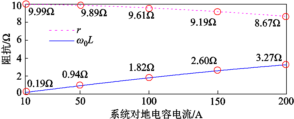
图4 等效阻抗数值
Fig.4 Equivalent impedance values
中性点小电阻投入后,零序网络如图5所示[22],小电阻投入后相应的电压与电流信号加上标“′”,i0z为流过中性点电流,Rz=3 RaZ。
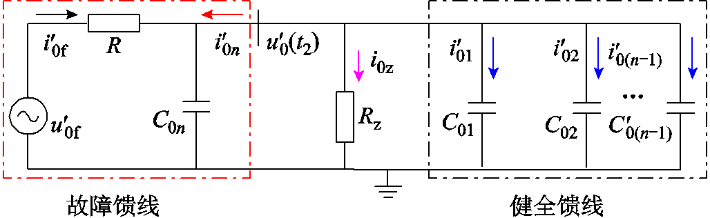
图5 小电阻接地系统零序网络
Fig.5 Zero sequence network of small resistance to ground system
根据图5,列写一阶微分方程为
 (7)
(7)
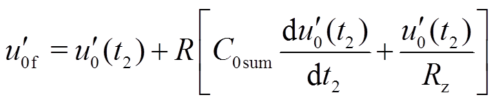
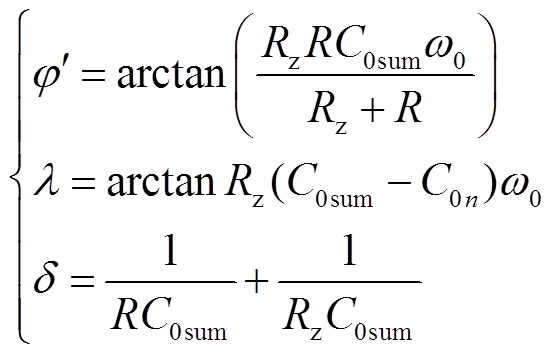
设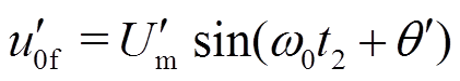 ,求解微分方程,可得母线零序电压为
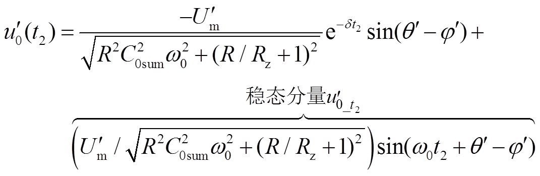 (8)
(8)
同时,可以计算出小电阻投入后中性点电流稳态分量 。
。
健全馈线零序电流为
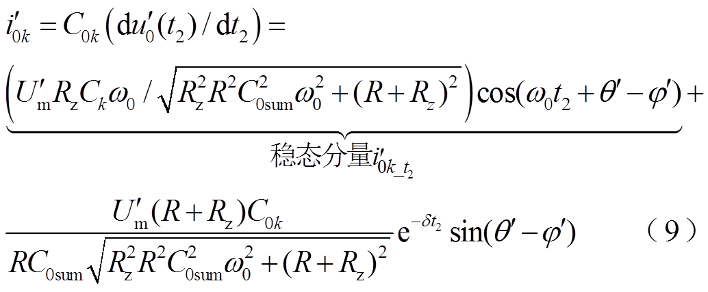
式中, 。
。
故障馈线零序电流为
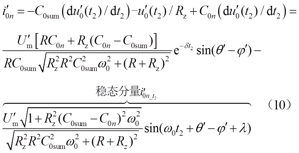
其中
对比式(9)与式(10),小电阻投入后, 幅值小于
幅值小于 的幅值,将在第2节与第3节进行详细分析。由于C0sum范围为1.84~36.8 μF,可以求解出0.017≤RzC0sumω0≤0.35,进而推导出λ近似变化范围为0.97°~19.29°,因此,与
 相位差为90.97°~119.29°。
对比式(4)与式(8),由于高阻故障时R/Rz远大于1,故 与
与 幅值关系为式(11),分析发现,R越大,与的幅值差越大。
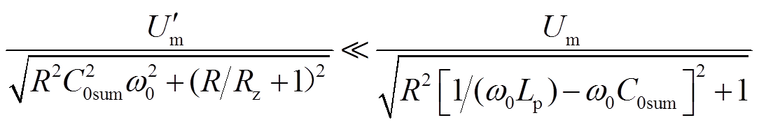 (11)
(11)
表1为高阻故障时,小电阻投入前后母线零序电压变化情况。由表1可知,小电阻投入后母线零序电压降落在95.3%~98.3%,电压下降得很明显。
表1 灵活接地系统母线电压降落
Tab.1 Bus voltage drop of flexible grounding systems

Rg/kΩu0/V压降(%) 0.56 21729095.3 1.05 16714997.1 1.54 39610097.7 2.03 8037498.1 2.53 3435998.2 3.02 9755098.3
为测试中性点小电阻投入前后不同时段下内积投影效果,给出灵活接地系统电压、电流如图6所示。图6为灵活接地系统发生1 kΩ高阻故障,故障时刻0.5 s,小电阻投入时刻为0.8 s,其中,零序电压互感器最小测量电压为120 V[18-19]。
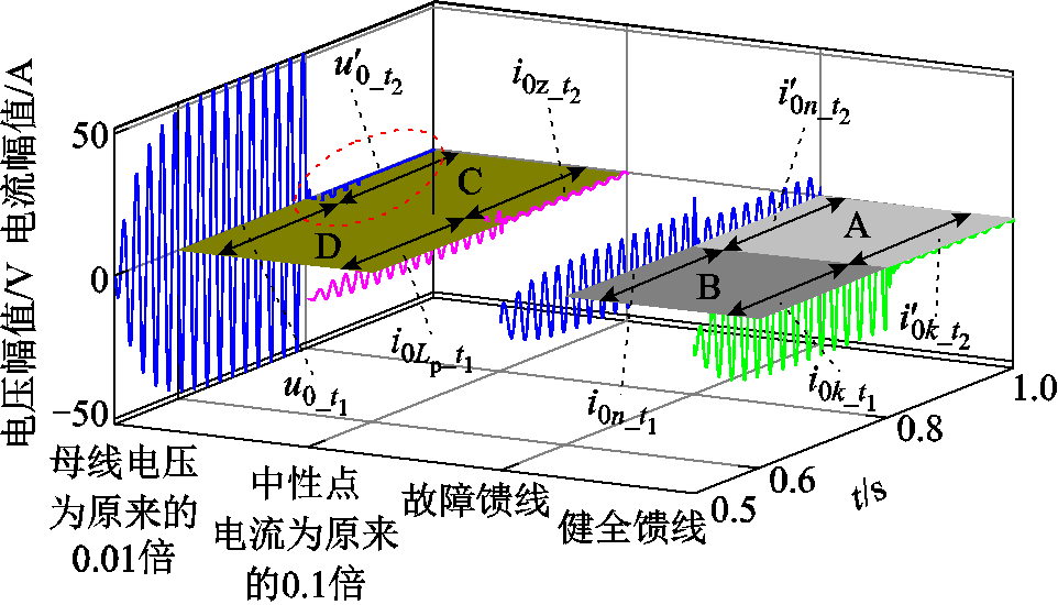
图6 灵活接地系统电压与电流
Fig.6 Flexible grounding system voltage and current
观察图6可知,小电阻的投入可将故障信号从时段上分为小电阻投入前与小电阻投入后,同时,考虑投影量与被投影量,可将图6电压、电流划分为A(,)、B(,)、C( ,)、D(
,)、D( ,)四部分,故存在四种内积投影可能:①A对C内积投影;②A对D内积投影;③B对C内积投影;④B对D内积投影。因此,分析不同时段下内积投影对高阻故障选线的适应性[2]。
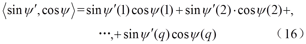
 内积投影
内积投影对做内积投影,有
式中, 为计算内积投影运算符号。
对做内积投影,有
当系统对地电容电流为200 A时, 36.8 μF,则λ=19.29°,并令
 =90°。由于单条馈线对地电容电流最大不超过50 A,由此,单条馈线对地电容Ck最大值为9.193μF,故Ckω0最大值为2.89 mS。当Rg变化范围为0~1 000 Ω,t2变化范围为3~4 s,同时考虑互感器最小测量电压为120 V,计算N1与N2,内积投影如图7所示。观察图7a与图7b可知,当接地电阻较小时,故障馈线内积投影值N1的幅值大于健全馈线内积投影值N2,二者在幅值上区分度较高;随着接地电阻增加,的幅值变小,电压信号幅值会受到互感器最小测量电压的限制,直观地表现在高阻故障时N1幅值与N2幅值差异较小。因此,若采用A对做内积投影将无法实现高阻故障的准确选线。
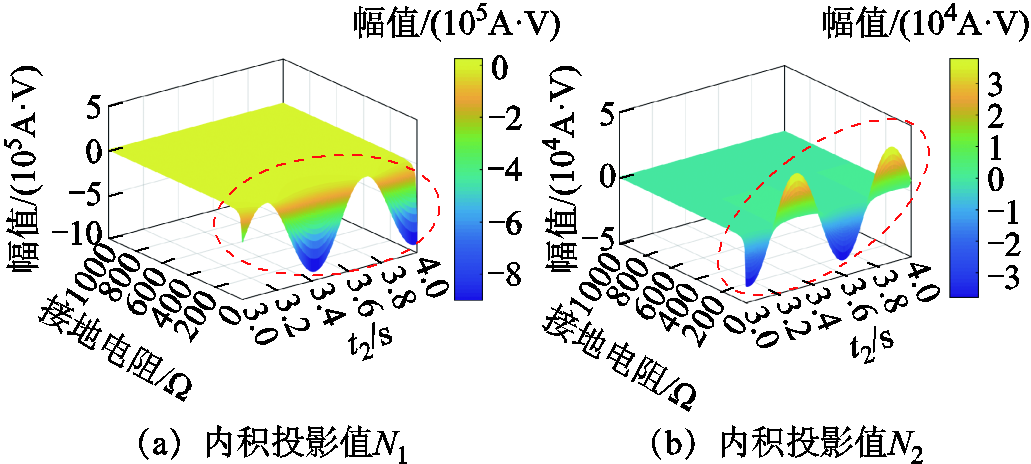
图7 内积投影
Fig.7 Inner product projection
 内积投影
内积投影发生接地故障时, 的幅值近似计算为
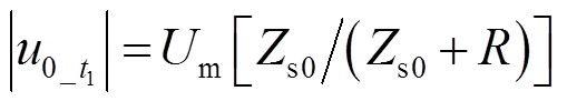 (14)
(14)
式中,Zs0为系统阻抗。谐振接地系统等效阻抗一般不小于1 700 Ω,Um取值为5 774 V。是唯一测量信号,当互感器最小测量电压为120 V时,可以根据式(14)推算出接地电阻为26 699 Ω,等同于Rg>26 699 Ω时,电压互感器精度不满足。因此,更适合作为被投影量。
与内积投影对比式(5)与式(6), 与
与 幅值差异部分为
 与
与 。当Ckω0取最大值2.89mS,Lp取最小值0.25 H时,取值为0.23。根据图3结论可以得出
 ,此时,的幅值大于。故B对与内积投影将无法实现故障馈线的检测。
依据图6,计算各时间尺度下内积投影结果如图8所示。从图8a与图8b内积投影幅值大小可以判别出故障馈线,但图8a内积投影幅值的阈值极小,如果Rg>1 000 Ω时,动作可靠性无法保证。观察图8c与图8d可知,其内积投影幅值差异明显,据此差异可以判别出故障馈线。进一步,分析图8e、图8f、图8g、图8h发现,健全馈线的内积投影幅值反而大于故障馈线,因此,故障馈线判别错误。
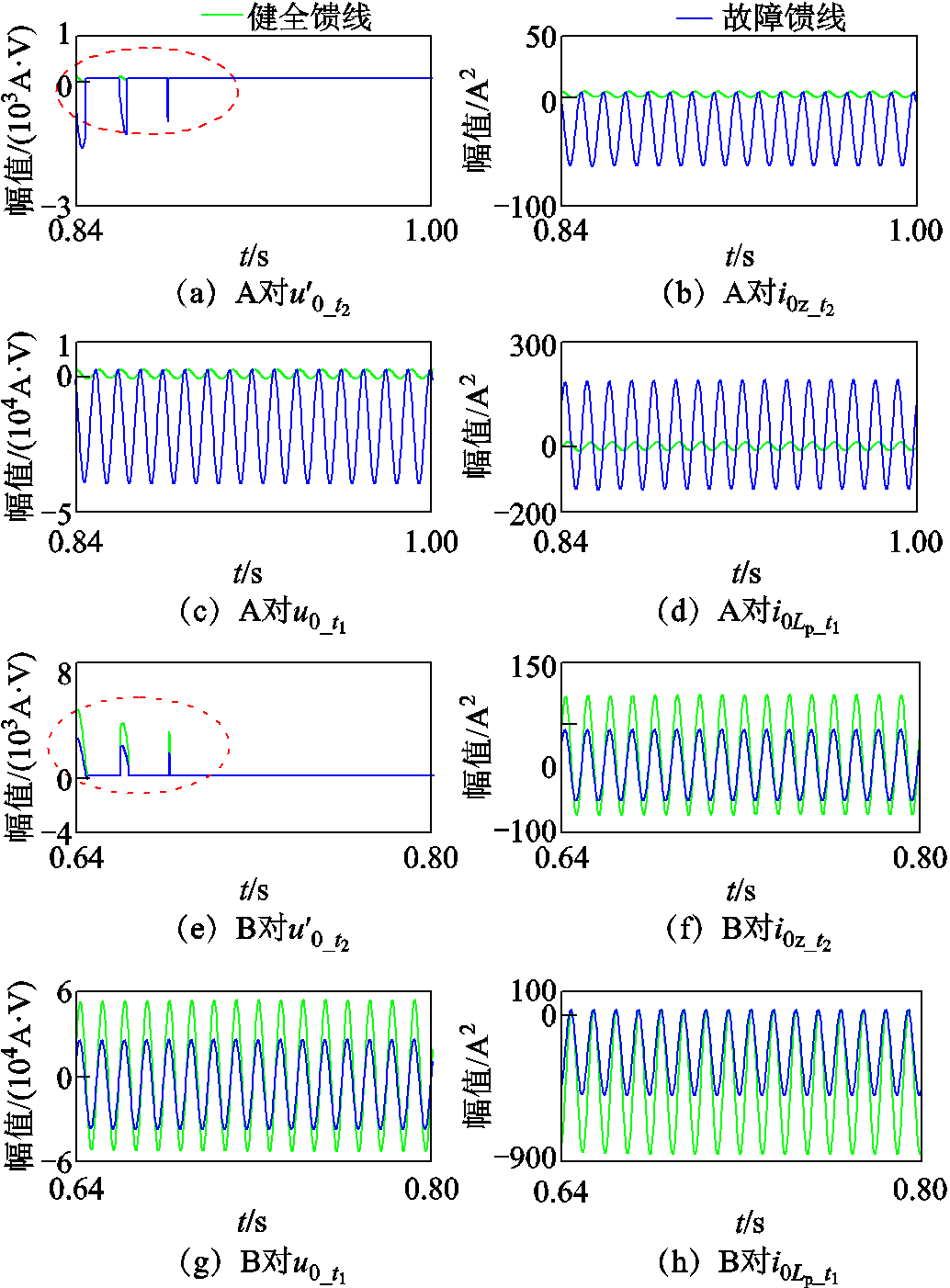
图8 各时段下内积投影
Fig.8 Inner product projection of each time period
综合理论推理与图8分析可得出以下结论:
(1)A( ,
, )对C(
)对C( ,)内积投影的差异随着接地电阻的增加而减小,故不适合高阻故障选线。B(,)对C(
 ,)与D(
,)与D( ,
, )内积投影的结果无法准确判定出故障馈线。
(2)A( ,)对D(,)内积投影结果在故障馈线与健全馈线之间存在明显幅值差异,因此,该内积投影方案适合作为高阻故障选线依据。
根据第1节与第2节分析结论,可得不同时段下内积投影原理如图9所示[20]。
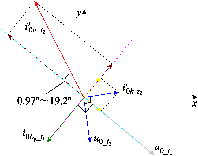
图9 内积投影原理
Fig.9 Inner product projection principle
由图9可知对与内积投影的幅值较大,对与 内积投影的幅值较小,具体不同时段内积投影计算如下。
对做内积投影,有
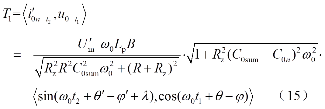
定义 ,
, ,则
,则 可表示为
可表示为
式中,q为数据窗采样点数量。当Rg=1 000 Ω,系统对地电容电流为200 A时, ,Lp=0.25 H,则
 ,
,  ,
,  ,并令
,并令 和
和 。从t1与t2时刻开始采样,采样频率100 Hz,q=100,可得内积投影如图10所示,进而可知取值范围为-56.56~56.56。
进一步,对做内积投影,有

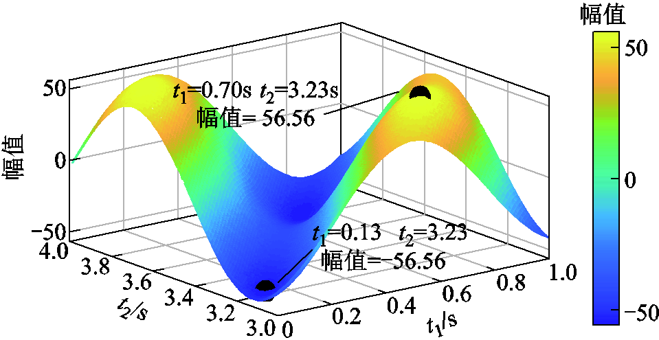
图10 sinψ′对cosψ做内积投影
Fig.10 Inner product projection of sinψ′ onto cosψ
计算 内积投影如图11所示,同理可知取值范围为-56.54~56.54。

图11 cos(ψ′ )对cosψ做内积投影
Fig.11 Inner product projection of cos(ψ′) onto cosψ
由此可见, 与
与
![]() 的取值范围基本相同,即
的取值范围基本相同,即
 (18)
(18)
因此,影响 、
、 大小的因素主要为
 、
、 。
。
当C0sum取值为1.84~36.8 μF时,有
 (19)
(19)
同时,由前文分析可知,单条馈线的C0kω0最大值为2.89 mS,则有
RzC0kω0≤0.087 (20)
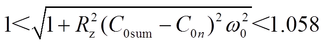
根据式(19)、式(20)的数值取值范围,可求出与的幅值范围,具体为
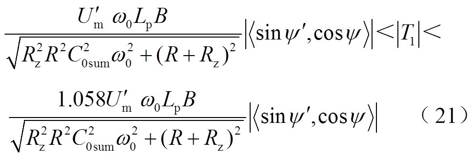
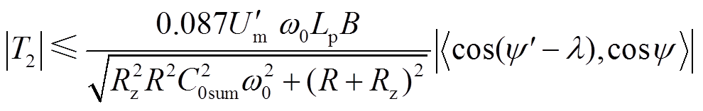 (22)
(22)
分析式(21)、式(22)可以得出, 。
。
同理,对 做内积投影,有
计算 的结果如图12所示,同理可知
 取值范围为-56.54~56.56。
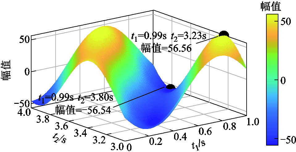
图12 sin(ψ′)对sin(ψ)做内积投影
Fig.12 Inner product projection of sin(ψ′) onto sin(ψ)
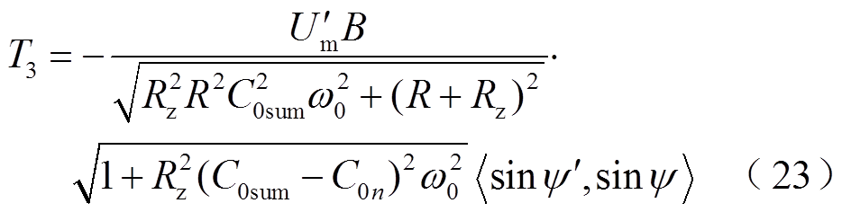
同理,对 做内积投影,有
 (24)
(24)
计算 内积投影如图13所示,可得取值范围为-56.56~56.56。
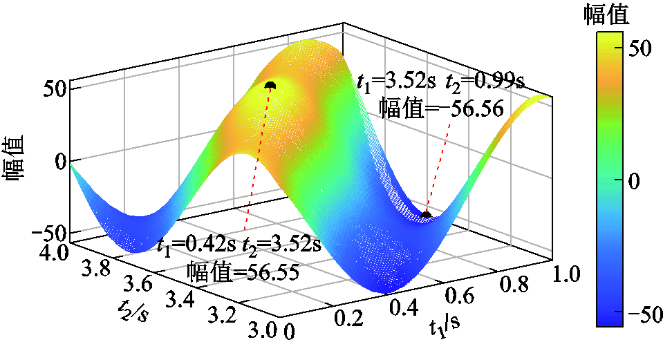
图13 cos(ψ′-λ)对sinψ做内积投影
Fig.13 Inner product projection of cos(ψ′-λ) onto sinψ
同理可知
 (25)
(25)
进一步, 、
、 的大小比较方式与
 、
、 完全相同,由此可知,
 。
。
因此,构建基于不同时段下内积投影的灵活接地系统高阻选线判据,具体如下:
(1)判据1:对、大小进行比较,若 ,判定出馈线n为故障馈线。
(2)判据2:对、大小进行比较,若 ,判定出馈线n为故障馈线。
(3)最终判定:当判据1与判据2判定结果一致时,判定最终故障馈线为馈线n;当判据1与判据2判定结果不一致时,对各馈线零序电流、母线零序电压、中性点电流进行重新采样,并再次进行判断,直到判定出最终故障馈线为止。
具体故障选线流程如图14所示,当接地电阻大于3 kΩ时,采用5%相电压启动。
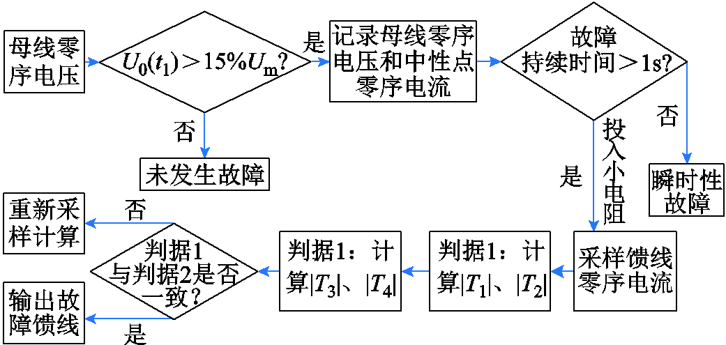
图14 故障选线流程
Fig.14 Fault line selection process
在PSCAD中搭建含DGs的辐射状灵活接地系统,验证方法的适应性[23]。辐射状灵活接地配电系统如图15所示,具体参数见表2。
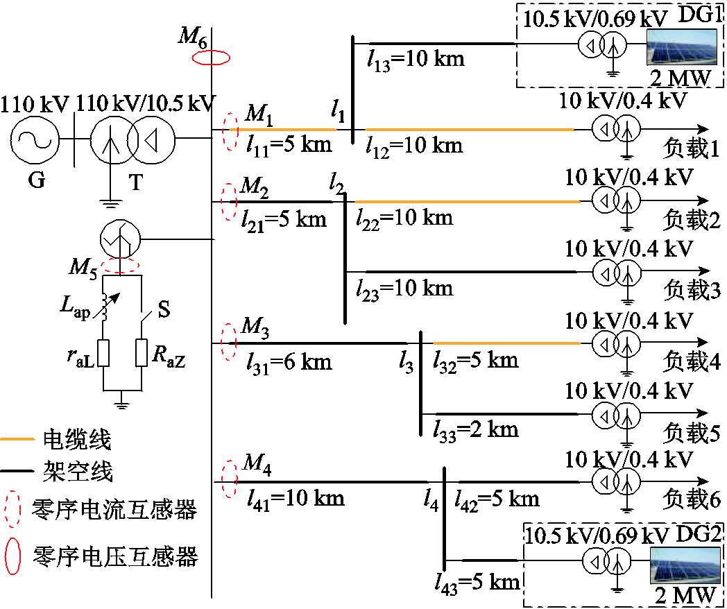
图15 辐射状灵活接地配电系统
Fig.15 Radial flexible grounding distribution systems
表2 灵活接地系统参数
Tab.2 The parameters of flexible grounding systems

设备类型参数 架空线路 R1: 0.170 0 Ω/km R0: 0.230 0 Ω/km 正序 L1: 1.200 0 mH/km零序 L0: 5.478 0 mH/km C1: 0.009 7 μF/km C0: 0.008 0 μF/km 电缆线路 R1: 0.270 0Ω/km R0: 2.700 0 Ω/km 正序 L1: 0.255 0 mH/km零序 L0: 1.019 0 mH/km C1: 0.339 0 μF/km C0: 0.280 0 μF/km 负载负载1~3:有功功率2.19 MW,无功功率0.39 Mvar 负载4~6:有功功率2.55 MW,无功功率0.45 Mvar 主变压器T正序漏抗: 0.000 01(pu)空载损耗: 0.000 62(pu) 短路损耗: 0.003 77(pu)额定功率: 31.5 MV·A 负载变压器正序漏抗: 0.100 00(pu)空载损耗: 0.001 15(pu) 短路损耗: 0.010 30(pu)额定功率: 3 MV·A DG变压器正序漏抗: 0.025 00(pu)额定功率: 2 MV·A Z型变压器漏抗: 0.100 00(pu)空载损耗: 0.003 40(pu) 短路损耗: 0.016 65(pu)额定功率: 0.2 MV·A 消弧线圈Lap: 0.348 3 H raL: 2.734 2 Ω (过补偿度10%) 小电阻RaZ: 10 Ω
对于灵活接地系统,仿真频率为10 kHz,工频为50 Hz,故障发生于0.5 s,小电阻投入时刻为1.5 s。
为有效避开小电阻投入瞬间产生的暂态扰动分量,该扰动分量一般持续2个工频周期,因此,选择时间尺度为1.540~1.545 s内的数据作为各条馈线零序电流的稳态分量。同理,将时间尺度为1.480~1.485 s内的数据作为中性点小电阻投入前的母线零序电压与中性点电流稳态分量。具体的时间尺度选择如图16a所示。
将各馈线零序电流分别对母线零序电压、中性点电流做内积投影,如图16b与图16c所示,可以看出,故障馈线l4内积投影幅值远大于健全馈线,且判据1与判据2判定结果相同,因此,将馈线l4判为故障馈线。
为进一步测试本文方法,分别从三种工况进行验证。
1)高阻工况。考虑不同故障馈线、故障距离D、故障初相位β、过补偿度γ、接地电阻Rg以噪声干扰。对本文方法进行验证,高阻故障判定结果见表3。从表3结果可以得出,在该类工况下,本文方法可以准确判定出故障馈线,即使在12 000 Ω接地电阻时,方法依然有效。
2)非同步采样(Asynchronous Sampling, AS)与数据缺失(Missing Data, MD)。图15验证了本文方法在非同步采样AS与数据缺失MD两种特殊故障工况下的适应性,具体工况见表4。
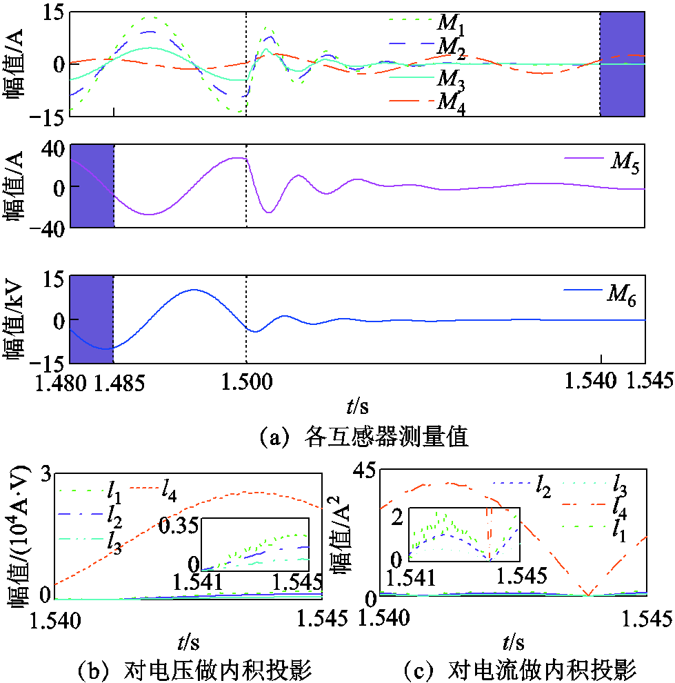
图16 不同时段选择与投影
Fig.16 Different time periods selection and projection
表3 高阻故障判定结果
Tab.3 Judgment results of high impedance fault
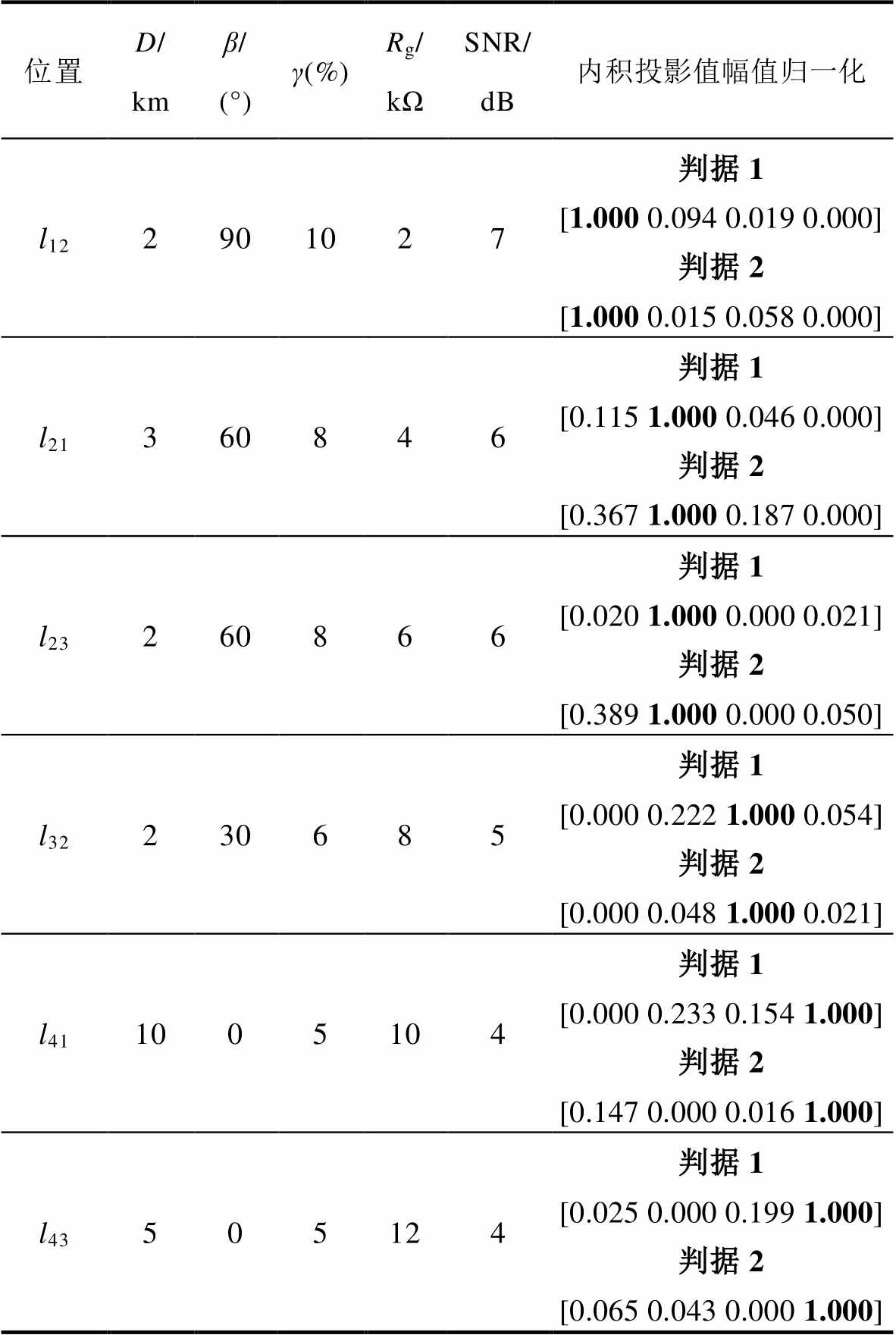
位置D/kmβ/ (°)γ(%)Rg/kΩSNR/ dB内积投影值幅值归一化 l122901027判据1 [1.000 0.094 0.019 0.000] 判据2 [1.000 0.015 0.058 0.000] l21360846判据1 [0.115 1.0000.046 0.000] 判据2 [0.367 1.000 0.187 0.000] l23260866判据1 [0.020 1.000 0.000 0.021] 判据2 [0.389 1.000 0.000 0.050] l32230685判据1 [0.000 0.222 1.000 0.054] 判据2 [0.000 0.048 1.000 0.021] l411005104判据1 [0.000 0.233 0.154 1.000] 判据2 [0.147 0.000 0.016 1.000] l43505124判据1 [0.025 0.000 0.199 1.000] 判据2 [0.065 0.043 0.000 1.000]
表4 非同步采样与数据缺失工况
Tab.4 Asynchronous sampling and missing data condition
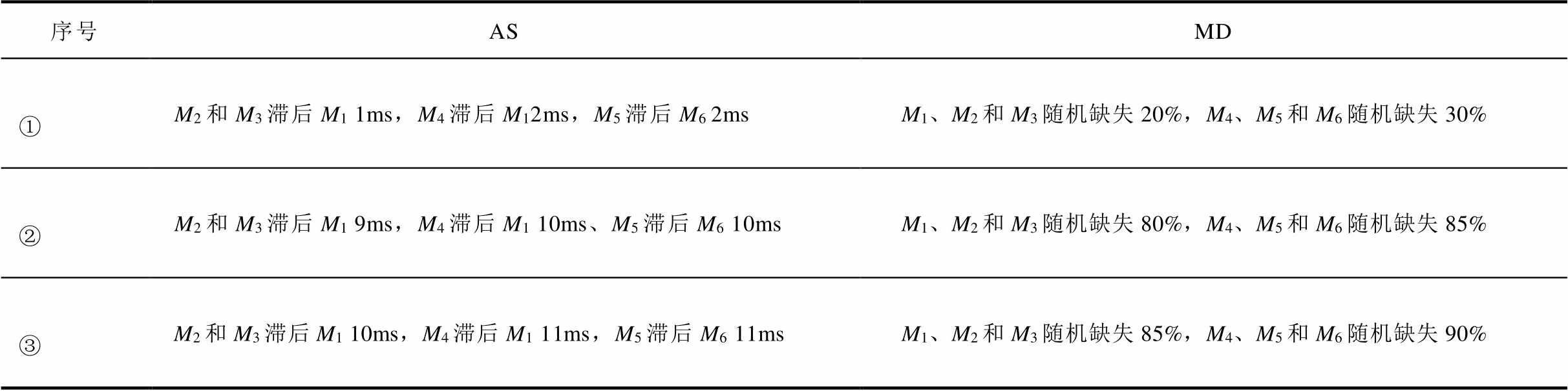
序号ASMD ①M2和M3滞后M1 1ms,M4滞后M12ms,M5滞后M6 2msM1、M2和M3随机缺失20%,M4、M5和M6随机缺失30% ②M2和M3滞后M1 9ms,M4滞后M1 10ms、M5滞后M6 10msM1、M2和M3随机缺失80%,M4、M5和M6随机缺失85% ③M2和M3滞后M1 10ms,M4滞后M1 11ms,M5滞后M6 11msM1、M2和M3随机缺失85%,M4、M5和M6随机缺失90%
馈线l4发生故障,同时发生非同步采样工况①与数据缺失工况①时,M1~M6波形如图17所示。
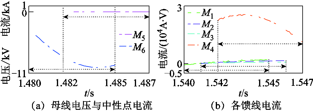
图17 非同步采样与数据缺失下电压、电流
Fig.17 Voltage and current under asynchronous sampling and missing data
对非同步采样与数据缺失工况进行测试,部分结果见表5。可以看出,该方法对非同步采样、数据缺失下的极端工况具有较高的准确性,即使数据缺失85%时,该方法依然有效。(由于方法判据1与判据2具有互补性,部分极端工况需重新采样计算才能判定出故障馈线,重新采样次数设定为3。)
表5 非同步采样与数据缺失时判定结果
Tab.5 Judgment results in case of asynchronous sampling and missing data

位置D/kmβ/(°)γ(%)Rg/kΩASMD内积投影值幅值归一化 l42590106①—[0.025 0.025 0.000 1.000] [0.254 0.156 0.000 1.000] l42590106②—[0.100 0.047 0.000 1.000] [0.274 0.206 0.000 1.000] l42590106③—[0.181 0.093 0.000 1.000] [0.341 0.206 0.000 1.000] l132055—①[1.000 0.044 0.021 0.000] [1.000 0.016 0.011 0.000] l132055—②[1.000 0.067 0.000 0.002] [1.000 0.034 0.000 0.001] l132055—③[0.000 0.036 1.000 0.004] [1.000 0.000 0.000 0.001] l21475108①①[0.158 1.000 0.050 0.000] [0.293 1.000 0.075 0.000]
3)电弧工况。采用Emanuel电弧模型验证该方法在非线性电弧时的适应性,电弧模型如图18所示。两个DC源Vp、Vn和两个二极管VDp、VDn组成正负半周电流路径;两个DC源Vp、Vn模拟电弧电压,其值取决于系统的电压水平与不对称建模,并且根据时间随机独立地变化;同时,通过两个电阻Rp、Rn取不同的值来模拟不对称电流。三种类型电弧参数见表6[24]。图19为三种案例时馈线首端电流与电压波形,可以看出,三种电流波形熄弧时间差异明显,并且案例3电流幅值最小;除此之外,小电阻投入后,母线电压明显下降,与式(11)分析结果一致。
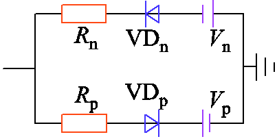
图18 Emanuel电弧模型
Fig.18 Emanuel arc model
表6 三种类型电弧参数
Tab.6 Three types of arc parameters
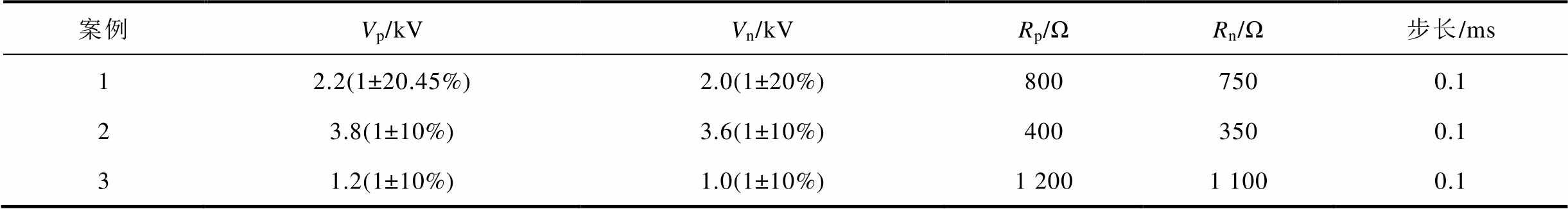
案例Vp/kVVn/kVRp/ΩRn/Ω步长/ms 12.2(1±20.45%)2.0(1±20%)8007500.1 23.8(1±10%)3.6(1±10%)4003500.1 31.2(1±10%)1.0(1±10%)1 2001 1000.1
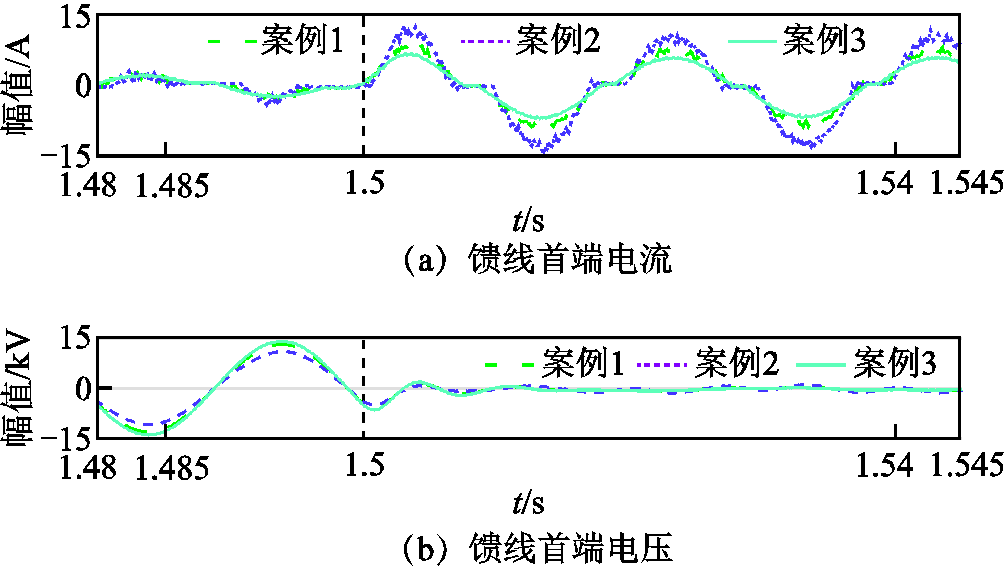
图19 电弧电流与电压
Fig.19 Arc current and voltage
在图15中模拟三种电弧案例,验证该方法的准确性。电弧故障时判定结果见表7。从表7中可以看出,在电弧故障时,本文方法可以准确判定出故障馈线。
表7 电弧故障时判定结果
Tab.7 Judgment results in case of arc fault

位置D/kmβ/(°)电弧案例内积值幅值归一化 l12801[1.000 0.004 0.001 0.000] [1.000 0.219 0.105 0.000] 2[1.000 0.037 0.016 0.000] [1.000 0.784 0.356 0.000]
(续)
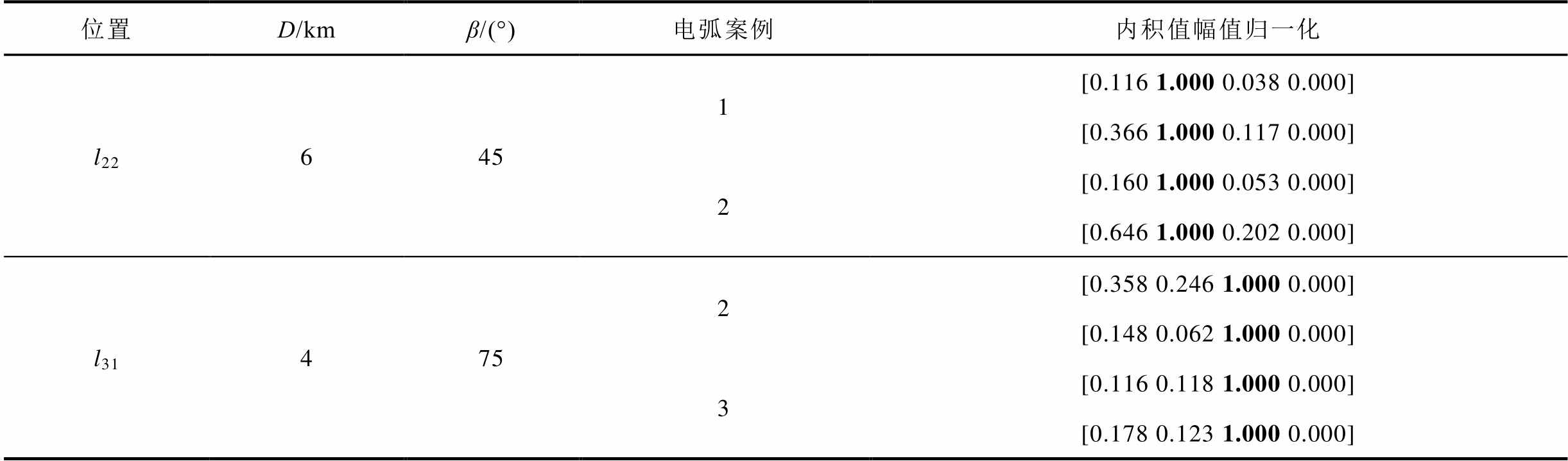
位置D/kmβ/(°)电弧案例内积值幅值归一化 l226451[0.116 1.000 0.038 0.000] [0.366 1.000 0.117 0.000] 2[0.160 1.000 0.053 0.000] [0.646 1.000 0.202 0.000] l314752[0.358 0.246 1.000 0.000] [0.148 0.062 1.000 0.000] 3[0.116 0.118 1.000 0.000] [0.178 0.123 1.000 0.000]
为进一步验证本文方法有效性,将本文方法与文献[19-20]进行比较。
根据第3节原理分析,本文方法使用不同时段内积投影的幅值作为故障馈线判定判据;而文献[19]采用各馈线电流与中性点电流的相位差对应的互相关系数构造判据;文献[20]仅依据小电阻投入前后馈线电流与母线电压之间的相位差变化量构造判据。依据图15灵活接地系统,采用表8所示故障工况进行对比分析,其中考虑了电流互感器反接。
表8 具体故障工况
Tab.8 Specific fault conditions

序号工况 1l43 D=5km β=30° γ=10% SNR=2dB 电弧案例3 2l21 D=2km β=60° γ=10% SNR=5dB 电弧案例2数据缺失:① 3工况1 M2反接 4l33 D=1km β=90° γ=5% SNR=3dB 电弧案例1M2与M3反接
电流互感器反接发生在中国湖南湘西某110 kV变电站,10 kV系统共计两段母线10条出线,网络拓扑结构如图20所示。
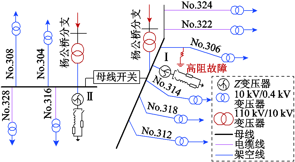
图20 现场测试的网络拓扑结构
Fig.20 Network topology of field test
当发生两种类型的高阻故障时,I母线的零序电流如图21所示,其中No.312、No.314、No.318、No.322、No.324为健全馈线,No.306为故障馈线。这两类高阻故障来自于No.306发生的两次接地故障。从图21可以看出,由于No.318电流互感器反接,波形与其他健全馈线的波形相反。

图21 现场测试数据
Fig.21 The field data
图22为工况4下零序电流互感器采用未反接与反接两种情形下的仿真结果。可以看出,当零序电流互感器M2与M3反接后,所测得的馈线l2、l3的零序电流波形发生了反向。需要注意的是,由于馈线l4为纯架空线,其对地电容数值较小,故M4测到的零序电流数值很小。如图21与图22结果所示,电流互感器反接后,馈线电流具有相同的相位变化。
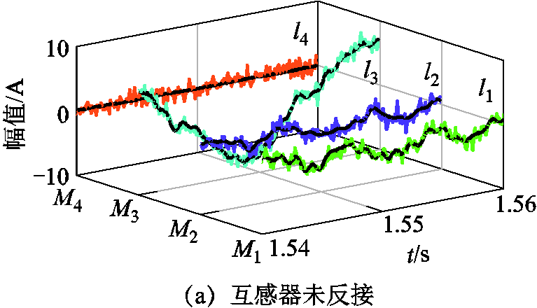
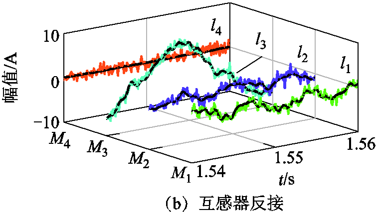
图22 零序电流互感器未反接与反接时所测电流
Fig.22 Current measured when the zero-sequence current transformers are unreversed and reversed
具体计算结果见表9~表11。从表9可以看出,本文方法在四种工况下仍然具有良好的稳定性,均可准确判定出故障馈线。从表10和表11可以看出,文献[19-20]方法均发生不同程度的误判现象,分析原因在于,消弧线圈的过补偿程度会直接影响健全馈线与故障馈线的相位特征,因此,基于相位变化量的故障判据在该种工况下极易发生误判。
表9 本文方法的判断结果
Tab.9 Judgment results of this paper method

序号判据1判据2结果 1[0.059 0.055 0.000 1.000] [0.228 0.281 0.000 1.000]l4 2[0.238 1.000 0.089 0.000] [0.176 1.000 0.056 0.000]l2 3[0.305 1.000 0.083 0.000][0.385 1.000 0.027 0.000]l2 4[0.292 0.111 1.000 0.000] [0.545 0.859 1.000 0.000]l3
表10 文献[19]方法判定结果
Tab.10 The judgment results of Ref.[19]

序号计算馈线[μ1,μ2,μ3,μ4]判据μj>μset(μset=35.30)选线结果是否正确 1[6.18 4.54 80.30 1.06]80.30>μsetl3错误 2[5.35 3.24 7.08 1.48]7.08<μset无故障错误 3[5.01 268.04 8.15 12.87]268.04>μsetl2正确 4[10.83 4.23 30.06 8.78]30.06<μset无故障错误
表11 文献[20]方法判定结果
Tab.11 The judgment results of Ref.[20]
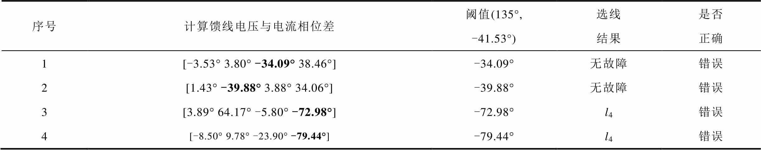
序号计算馈线电压与电流相位差阈值(135°,-41.53°)选线结果是否正确 1[-3.53° 3.80° -34.09°38.46°]-34.09°无故障错误 2[1.43°-39.88°3.88° 34.06°]-39.88°无故障错误 3[3.89° 64.17° -5.80° -72.98°]-72.98°l4错误 4[-8.50° 9.78° -23.90° -79.44°]-79.44°l4错误
进一步地,为测试本文方法与现有方法的计算时间。经测算可知,本文方法平均耗时0.05 s,而文献[19-20]方法分别耗时0.26 s、0.38 s。由此可见,本文方法在判定时间方面也具有明显优势。
通过研究,得出以下结论:
1)灵活接地系统在小电阻投入前为谐振接地系统,投入后可等效为小电阻接地系统,并且小电阻投入后故障馈线零序电流稳态分量幅值显著大于健全馈线;同时,小电阻投入后母线零序电压会发生降低现象。因此,小电阻投入前的母线零序电压更适合作为被投影量。
2)本文方法将小电阻投入后各馈线零序电流对小电阻投入前母线零序电压与中性点电流的内积投影相结合,构造了两种故障馈线判据,充分利用不同时段下的故障特征,提高了高阻故障选线的准确性。
3)在含DGs的辐射状灵活接地系统中,验证了不同类型工况,均表明本文方法具有较好的适应性;与基于相位的选线判据相比,本文方法适应复杂工况能力更强,且判据的计算时间最短;除此之外,本文方法在电流互感器反接时,依然可以准确判定出故障馈线。
参考文献
[1] 刘宝稳, 曾祥君, 张慧芬, 等. 不平衡零序电压快速精准抑制与电压消弧全补偿优化控制方法[J]. 电工技术学报, 2022, 37(3): 645-654. Liu Baowen, Zeng Xiangjun, Zhang Huifen, et al. Optimal control method for accurate and fast suppression of unbalanced zero-sequence voltage and voltage arc suppression full compensation[J]. Transactions of China Electrotechnical Society, 2022, 37(3): 645-654.
[2] Wang Xiaowei, Liu Weibo, Liang Zhenfeng, et al. Faulty feeder detection based on the integrated inner product under high impedance fault for small resistance to ground systems[J]. International Journal of Electrical Power & Energy Systems, 2022, 140: 108078.
[3] Liu Penghui, Du Shaotong, Sun Kang, et al. Single-line-to-ground fault feeder selection considering device polarity reverse installation in resonant grounding system[J]. IEEE Transactions on Power Delivery, 2021, 36(4): 2204-2212.
[4] 王宾, 崔鑫. 基于伏安特性动态轨迹的谐振接地系统弧光高阻接地故障检测方法[J]. 中国电机工程学报, 2021, 41(20): 6959-6968. Wang Bin, Cui Xin. Detection method of arc high resistance grounding fault in resonant grounding system based on dynamic trajectory of volt-ampere characteristic[J]. Proceedings of the CSEE, 2021, 41(20): 6959-6968.
[5] 杨帆, 刘鑫星, 沈煜, 等. 基于零序电流投影系数的小电阻接地系统高阻接地故障保护[J]. 电网技术, 2020, 44(3): 1128-1133. Yang Fan, Liu Xinxing, Shen Yu, et al. High resistance ground fault protection of low resistance grounding system based on zero sequence current projection coefficient[J]. Power System Technology, 2020, 44(3): 1128-1133.
[6] 王晓卫, 高杰, 吴磊, 等. 柔性直流配电网高阻接地故障检测方法[J]. 电工技术学报, 2019, 34(13): 2806-2819. Wang Xiaowei, Gao Jie, Wu Lei, et al. A high impedance fault detection method for flexible DC distribution network[J]. Transactions of China Electrotechnical Society, 2019, 34(13): 2806-2819.
[7] Wei Xiangxiang, Wang Xiaowei, Gao Jie, et al. Faulty feeder detection for single-phase-to-ground fault in distribution networks based on transient energy and cosine similarity[J]. IEEE Transactions on Power Delivery, 2022, 37(5): 3968-3979.
[8] 邓丰, 梅龙军, 唐欣, 等. 基于时频域行波全景波形的配电网故障选线方法[J]. 电工技术学报, 2021, 36(13): 2861-2870. Deng Feng, Mei Longjun, Tang Xin, et al. Faulty line selection method of distribution network based on time-frequency traveling wave panoramic waveform[J]. Transactions of China Electrotechnical Society, 2021, 36(13): 2861-2870.
[9] 喻锟, 胥鹏博, 曾祥君, 等. 基于模糊测度融合诊断的配电网接地故障选线[J]. 电工技术学报, 2022, 37(3): 623-633. Yu Kun, Xu Pengbo, Zeng Xiangjun, et al. Grounding fault line selection of distribution networks based on fuzzy measures integrated diagnosis[J]. Transactions of China Electrotechnical Society, 2022, 37(3): 623-633.
[10] Liu Kangli, Zhang Sen, Li Baorun, et al. Flexible grounding system for single-phase to ground faults in distribution networks: a systematic review of developments[J]. IEEE Transactions on Power Delivery, 2022, 37(3): 1640-1649.
[11] 刘宝稳, 曾祥君, 张慧芬, 等. 有源柔性接地配电网弧光高阻接地故障检测方法[J]. 中国电机工程学报, 2022, 42(11): 4001-4013. Liu Baowen, Zeng Xiangjun, Zhang Huifen, et al. Arc high resistance grounding fault detection method for active flexible grounding distribution network[J]. Proceedings of the CSEE, 2022, 42(11): 4001-4013.
[12] Tang Jinrui, Xiong Binyu, Li Yang, et al. Faulted feeder identification based on active adjustment of arc suppression coil and similarity measure of zero-sequence currents[J]. IEEE Transactions on Power Delivery, 2021, 36(6): 3903-3913.
[13] Wang Yuanyuan, Chen Qiaoshan, Zeng Xiangjun, et al. Faulty feeder detection based on space relative distance for compensated distribution network with IIDG injections[J]. IEEE Transactions on Power Delivery, 2021, 36(4): 2459-2466.
[14] 薛永端, 金鑫, 刘晓, 等. 灵活接地系统中配电网接地保护的适应性分析[J]. 电力系统自动化, 2022, 46(5): 112-121. Xue Yongduan, Jin Xin, Liu Xiao, et al. Analysis on adaptability of grounding protection for distribution network in flexible grounded system[J]. Automation of Electric Power Systems, 2022, 46(5): 112-121.
[15] 杨帆, 任伟, 沈煜, 等. 消弧线圈并联小电阻系统接地故障灵活处理策略[J]. 供用电, 2019, 36(3): 44-49. Yang Fan, Ren Wei, Shen Yu, et al. Grounding fault processing strategy in petersen coil paralleled small resistance grounding system[J]. Distribution & Utilization, 2019, 36(3): 44-49.
[16] 尹力, 孔令昌, 王冠华, 等. 基于负序电压变化量的灵活接地配电网永久性单相接地故障定位[J]. 电力自动化设备, 2023, 43(1): 83-89, 99. Yin Li, Kong Lingchang, Wang Guanhua, et al. Permanent single-phase grounding fault location in flexible grounding distribution network based on negative-sequence voltage variation[J]. Electric Power Automation Equipment, 2023, 43(1): 83-89, 99.
[17] 王义凯, 尹项根, 乔健, 等. 协同多模接地控制的海洋核动力平台电网接地故障选线方法[J]. 电力自动化设备, 2022, 42(11): 176-182. Wang Yikai, Yin Xianggen, Qiao Jian, et al. Grounding fault line selection method coordinated with multi-mode grounding control for power grid of marine nuclear power platform[J]. Electric Power Automation Equipment, 2022, 42(11): 176-182.
[18] 杨帆, 金鑫, 沈煜, 等. 基于零序导纳变化的灵活接地系统接地故障方向判别算法[J]. 电力系统自动化, 2020, 44(17): 88-94. Yang Fan, Jin Xin, Shen Yu, et al. Dicrimination algorithm of grounding fault direction based on variation of zero-sequence admittance in flexible grounding system[J]. Automation of Electric Power Systems, 2020, 44(17): 88-94.
[19] 刘朋跃, 邵文权, 弓启明, 等. 利用零序电流相位变化特征的灵活接地系统故障选线方法[J]. 电网技术, 2022, 46(5): 1830-1838. Liu Pengyue, Shao Wenquan, Gong Qiming, et al. Fault line detection of flexible grounding system based on phase variation characteristics of zero-sequence current[J]. Power System Technology, 2022, 46(5): 1830-1838.
[20] 李建蕊, 李永丽, 王伟康, 等. 基于零序电流与电压相位差变化的灵活接地系统故障选线方法[J]. 电网技术, 2021, 45(12): 4847-4855. Li Jianrui, Li Yongli, Wang Weikang, et al. Fault line detection method for flexible grounding system based on changes of phase difference between zero sequence current and voltage[J]. Power System Technology, 2021, 45(12): 4847-4855.
[21] 叶远波, 汪胜和, 谢民, 等. 高阻接地故障时消弧线圈并联小电阻接地的控制方法研究[J]. 电力系统保护与控制, 2021, 49(19): 181-186. Ye Yuanbo, Wang Shenghe, Xie Min, et al. Study on the control method of high impedance faults in the neutral via arc suppression coil paralleled with a low resistance grounded system[J]. Power System Protection and Control, 2021, 49(19): 181-186.
[22] 王宾, 崔鑫, 董新洲. 配电线路弧光高阻故障检测技术综述[J]. 中国电机工程学报, 2020, 40(1): 96-107, 377. Wang Bin, Cui Xin, Dong Xinzhou. Overview of arc high impedance grounding fault detection technologies in distribution system[J]. Proceedings of the CSEE, 2020, 40(1): 96-107, 377.
[23] 秦苏亚, 薛永端, 刘砾钲, 等. 有源配电网小电流接地故障暂态特征及其影响分析[J]. 电工技术学报, 2022, 37(3): 655-666. Qin Suya, Xue Yongduan, Liu Lizheng, et al. Transient characteristics and influence of small current grounding faults in active distribution network[J]. Transactions of China Electrotechnical Society, 2022, 37(3): 655-666.
[24] Gao Jie, Wang Xiaohua, Wang Xiaowei, et al. A high-impedance fault detection method for distribution systems based on empirical wavelet transform and differential faulty energy[J]. IEEE Transactions on Smart Grid, 2022, 13(2): 900-912.
Abstract High impedance faults are a common form of distribution network faults, accounting for about 5% to 10% of medium voltage distribution network faults, often accompanied by arcing, which can easily cause safety hazards. Due to the weak fault characteristics of high impedance faults, most faulty feeder detection methods only have high accuracy for low-impedance faults. This is insufficient to support the principle of proximity and fast isolation of ground faults. Recently, some high impedance fault line selection methods have been proposed, but most of them suffer from complex principles, single criteria, and equipment measurement accuracy that does not meet the demand. To address these problems, this paper proposed high impedance fault line selection methods based on inner product projection of different time periods for flexible grounding systems. It can accurately detect the faulty feeder at high impedance faults through the characteristic quantities of voltage and current before and after small resistance input.
Firstly, the inner product projection of each feeder’s zero-sequence current after small resistance input onto the bus zero-sequence voltage before small resistance input is constructed as criteria 1. Secondly, the inner product projection of each feeder’s zero-sequence current after small resistance input onto the neutral point zero-sequence current before small resistance input is constructed as criteria 2. Finally, when the results of the faulty feeder determined by criterion 1 and criterion 2 are the same, the final faulty feeder result is obtained. The fault detection method fully uses the fault characteristics under different time periods, solves the influence of bus zero-sequence voltage drop after small resistance input and a single criterion on the detection accuracy, and greatly simplifies the faulty feeder detection principle, resulting in a highly accurate faulty feeder detection method.
The simulation results using a flexible grounding system show that. Firstly, the faulty feeder can be accurately determined under high impedance fault conditions considering different fault feeders, fault distance, fault initial phase angle, overcompensation, ground resistance and noise interference. Second, considering asynchronous sampling and missing data, where asynchronous sampling is up to 11ms and data missing is up to 85%, the proposed method still has good stability. Then, the accuracy of the proposed method is verified under three arc parameters. Finally, the proposed method is compared with two flexible grounding system methods under four complex operating conditions, where a current transformer reversal was considered, the proposed method takes the shortest time of 0.05 s, and there is no misjudgment.
The following conclusions can be drawn from the simulation analysis: (1) Compared with existing methods, the proposed method greatly simplifies the principle of detection criterion and effectively overcomes the bus zero-sequence voltage reduction problem. Therefore, it is appropriate to use different time periods of fault characteristics. (2) The proposed method combines the inner product projection of each feeder current after small resistance input onto the bus voltage and neutral point current before small resistance input. It uses two types of criteria, both of which complement each other to improve the accuracy of fault feeder determination. (3) The proposed method is more capable of adapting to complex working conditions, and the calculation time of the criterion is short. In addition, the faulty feeder can still be accurately determined when the current transformer is reversed.
keywords:Flexible grounding systems, high impedance fault, different time periods, inner product projection
DOI:10.19595/j.cnki.1000-6753.tces.221878
中图分类号:TM77
国家自然科学基金项目(52177114, 61403127)和国网江西省电力有限公司科技项目(521820220016, 521820210005)资助。
收稿日期 2022-10-07
改稿日期 2022-11-30
王晓卫 男,1983年生,博士,副教授,博士生导师,研究方向为配电网故障选线与定位、高阻故障检测、电力工程信号处理。E-mail:proceedings@126.com(通信作者)
刘伟博 男,1997年生,硕士研究生,研究方向为新型配电系统高阻故障选线。E-mail:Lwei_bo@126.com
(编辑 赫 蕾)