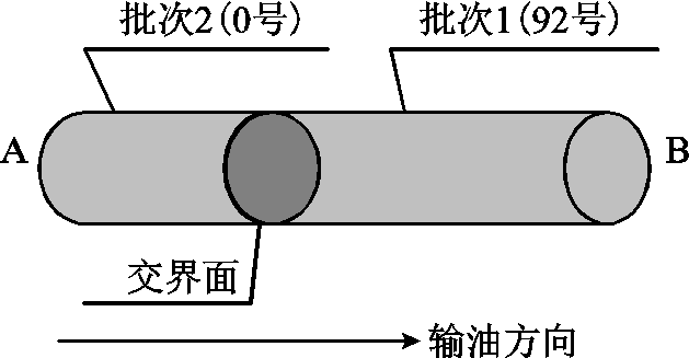
图1 成品油输送示意图
Fig.1 Schematic diagram of refined oil transportation
摘要 成品油管网具有多批次顺序输送特性,其管道网络参数为连续时变变量,导致压力约束中存在多个连续时变变量相乘项,具有很强的非线性。为此,该文借鉴流体力学中描述流体运动的思路,首先,将建模视角从传统基于欧拉法的管网视角切换到基于拉格朗日法的批次视角对模型进行等价重构以降低非线性;然后,综合大M法、分段线性化和二维凸组合等多种线性化技术进一步消除非线性,将非线性模型转换为易于求解的混合整数线性规划模型;最后,进行算例分析,结果表明所提模型较现有模型更能反映管网的复杂工况,在确保运输安全的同时提高经济性,其中电力成本降低27.95%,平均近似误差从19.74%降低至0.61%。
关键词:多批次输送 线性化技术 电力成本 输油节能
石油是重要的能源载体之一,其安全运输与人民生活息息相关,对于保障能源供应和能源安全具有十分重要的意义[1-2]。近年来,我国的石油运输行业稳步发展,2020年全国成品油输送管道建设总长度达3.2万km。然而,成品油运输行业在布局逐渐完善的同时也带来了大量的能源消耗和碳排放[3]。随着我国“双碳”目标的确立,开展成品油管网运输节能降耗的研究势在必行[4]。
成品油的运输过程以输油站场内主输泵及其他辅助设施为能耗主体[5]。以华南地区某成品油管线为例,其2019年输油量超3100万t/年,泵的耗电量约4.2万kW·h/年,“十四五”期间(2021—2025年)耗电量预计高达6亿kW·h。与此同时,管道运行过程中的节能优化潜力巨大,单台泵的节能效果累积起来可使电力成本和碳排放量大大减少[6]。因此,开展成品油管网的泵群决策研究来优化成品油管网的压力分布显得尤为必要[7]。
与城市输水管道类似[8],成品油的运输过程决策分为两个阶段:第一阶段为流量计划制定阶段,通常由计划部门根据下游市场需求来制定输油首站的注入油品种类和各个管段的流量来保证下游市场需求能够被及时满足[9];第二阶段为压力计划制定阶段,通常由调度部门根据已有的输油计划来制定相应的开泵方案。由于油品在传输过程中存在沿程摩阻和高程压降,因此需要在输油站场通过电动离心泵加压确保油品运输过程中各个节点的压力在安全范围内变化[10]。
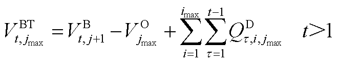
与输送单一介质的城市输水管道不同,成品油管网顺序输送多种介质。如图1所示,在一根管段AB内的某一时刻同时存在多种油品(如我国的0号柴油、92号汽油和95号汽油),并在中间下载站或末站完成分离。这种管道内同时存在多种介质的工况被定义为多批次特性,其中介质间交界面可以被简化为平面[6]。在本文中,对于前行油品批次1,交界面被定义为批次1的油尾;对于后行油品批次2,交界面被定义为批次2的油头。由于成品油管网存在特殊的多批次输送特性,其管道网络参数(例如油品密度和粘度)为连续时变变量,导致优化模型中存在多个连续时变变量相乘项,具有很强的非线性,难以求解[11]。
图1 成品油输送示意图
Fig.1 Schematic diagram of refined oil transportation
因此,现有研究大多将流量和压力进行变量解耦,对两阶段分别进行优化。如文献[12]针对下游市场需求搭建了多分叉的管网模型,同时考虑批次追踪、注入、下载和库存等约束,以最小泵耗、污染、库存和管道利用率等相关变量构建目标函数来决策流量计划,实现第一阶段的成本最小;文献[13]基于既定的批次计划,将流量视为已知常数,分析了运行开泵阶段的水力约束,以电力成本和起停成本最小为目标函数,用模型预测算法进行实时开泵决策,实现第二阶段电力成本最小。上述文献重点优化两阶段中的一个而将另一个阶段的变量视为既定常数,以实现成品油管道的优化调度。尽管上述方法将多批次模型的非线性项进行简化后易于求解,但是仅考虑单一阶段的约束存在两方面的弊端:一方面,仅考虑流量计划制定的模型可能在实际调度过程中出现压力越限造成无解的情况[14-16];另一方面,仅考虑压力计划制定的模型无法充分利用成品油管网的潜在灵活性,使泵群的电力成本降低空间有限[17-18]。
此外,也有部分学者针对两阶段联合优化提出了简化模型。文献[19]证明了管段的泵送速率越稳定,泵送油品的压力损失就越低,以每个管段泵送速率最小为目标函数进行两阶段联合求解。但该方法仅追求压力损失最小,无法反映电力成本变化;文献[20]提出压力控制模式下两阶段联合求解的混合整数线性规划模型,利用不同油品的特性平均值来线性化模型。但该方法对压力损失的近似较为粗略,对于长距离和高程压降较大的管段可能由于压力损失的近似误差造成压力越限;文献[21]将每个开泵方案下的压力约束与流量约束相关联,用流量约束来近似压力约束的启发式方法构建了两阶段联合求解的混合整数线性规划模型。但该方法没有对成品油管网的压力分布进行定量刻画,仅保障了第一阶段的安全而忽略了调度过程中压力变化的复杂工况。综上所述,现有的两阶段联合优化方法在一定程度上降低了电力成本,然而其对多批次复杂工况下两阶段联合优化模型中压力分布的近似误差仍然较大,难以在实际调度过程中决策出安全且经济的泵群调度方案。
针对上述分析,本文提出了基于压力约束重构的两阶段联合优化模型。本文主要工作与已有工作区别如下:
1)与现有建模方法不同,本文借鉴流体力学中描述流体运动的思路[22],将建模视角从传统基于欧拉法的管网视角切换到基于拉格朗日法的批次视角。在不损失模型精度的情况下,将压力约束中的连续时变变量等价重构为离散取值变量来降低模型非线性;同时将部分难以定量刻画的变量等价重构为易于表达且具备直观物理意义的新变量。
2)针对重构后的模型,本文进一步利用大M法、分段线性化和二维凸组合等多种线性化技术消除模型的非线性。在实际工程误差可接受的范围内,将两阶段联合优化模型转换为易于求解的混合整数线性规划模型。
3)本文将所提模型应用于国内西南地区某成品油输送管网,通过和现有模型的调度方案对比验证了所提模型在实际工业现场的适用性。
本节在文献[20]所提流量计划制定模型基础上,加入了基于传统管网视角的压力分布相关约束,并以最小化电力成本为目标函数构建两阶段联合优化模型。
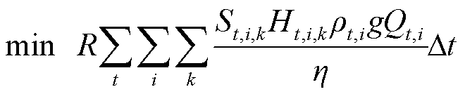
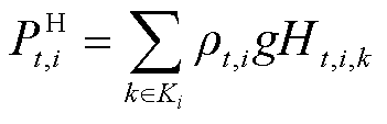
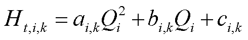
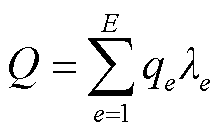
目标函数代表调度周期内所有站场主输泵的总电力成本,即
 (1)
(1)
式中,R为电价,本文取固定电价0.85 ¥/(kW·h); 为第t个时间窗内第
![]() 个站场第
个站场第![]() 台泵起停状态的0-1变量;
台泵起停状态的0-1变量; 为第
为第 个时间窗内第
 个站场过站油品密度;
 为第个时间窗内第个站场第
![]() 台主输泵的扬程;
台主输泵的扬程;![]() 为当地重力加速度,本文取9.81 m/s2;
为当地重力加速度,本文取9.81 m/s2;![]() 为站场的过站流量;
为站场的过站流量; 为泵效率,本文取
 ;
; 为调度时间窗长度,本文取
 。
。
值得注意的是,从管网视角构建的目标函数中存在多个连续变量相乘项,属于典型的NP-hard问题,难以直接求解[23]。
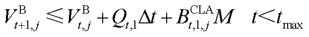
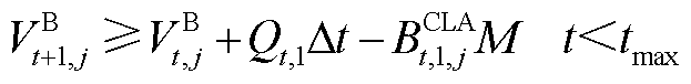
1)管段压力约束
 (2)
(2)
 (3)
(3)
 (4)
(4)
式中, 和
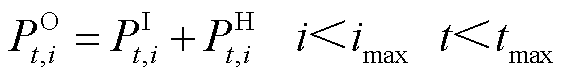
和 分别为站场进、出站压力;
 为站场主输泵所提供压力;
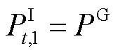
 为输油首站节点压力,本文取0.3 MPa,认为首站节点为恒压源[24];
 为第t个时间窗内管段
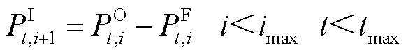
 内的压力损失。式(2)描述了过站前后压力变化,式(4)的含义是油品在管段传输过程中产生的压力损失变化。
2)压力损失约束
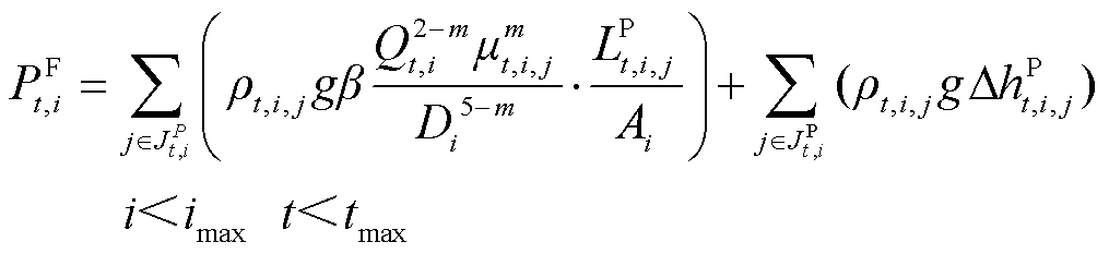 (5)
(5)
式中, 为第t个时间窗内管段内含有的所有油品批次集合;
 和
和 分别为第
分别为第![]() 个时间窗内第
个时间窗内第![]() 批次油品在管段的油品密度和粘度;
批次油品在管段的油品密度和粘度;![]() 和
和![]() 为列宾宗公式(Leapienzon formula)系数[10],本文分别取值为0.25和0.024 6;
为列宾宗公式(Leapienzon formula)系数[10],本文分别取值为0.25和0.024 6;![]() 为管段内径;Ai为管段横截面积;
为管段内径;Ai为管段横截面积; 为油品在管段内的体积;
 为油品在管段内的首末高程差。式(5)是在列宾宗公式[25]基础上从传统管网视角描述压力损失的表达式。
与目标函数类似,压力损失表达式中同样存在强非线性。此外,传统管网视角建模下的变量和难以用显示表达式进行描述。
3)泵站压力约束
泵站提供压力约束为
 (6)
(6)
 (7)
(7)
式中, 为第个站场主输泵集合;
 、
、 、
、 为第个站场第k台主输泵的扬程-流量特性系数[18]。
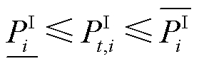
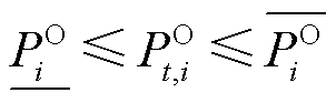
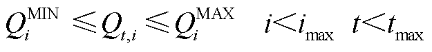
泵站进出站压力上下限约束为
 (8)
(8)
 (9)
(9)
式中, 和
和 分别为第个站场进站压力上、下限;
 和
和 分别为第个站场出站压力上、下限。
流量分布约束包括用于追踪不同批次油头和油尾的批次追踪约束、站场流量下载约束和管段流量耦合约束,具体公式见附录,约束的具体含义见文献[20]。
本节将建模视角从传统基于拉格朗日法的管网视角切换到基于欧拉法的批次视角,对目标函数和压力分布约束进行表达式重构,以降低模型非线性。
针对多批次油品的密度和粘度,在管网视角下二者为连续时变变量。而在批次视角下,二者可以被视为常数(即取值空间为0号柴油、92号汽油或95号汽油参数)。为此,本文提出二进制表示法,将目标函数式(1)和压力约束式(5)、式(6)中的密度和粘度这两个连续变量等价重构为离散取值变量来降低非线性。
以式(6)为例,重构过程为
 (10)
(10)
 (11)
(11)
 (12)
(12)
 (13)
(13)
 (14)
(14)
 (15)
(15)
式中, 和
和 为辅助的0-1变量;
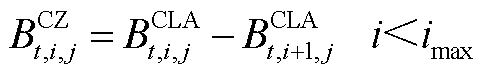
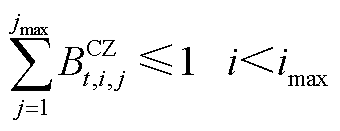
 为第t个时间窗内第j批次油头已到达第i个站场且油尾尚未到达第i个站场的状态变量,若满足则
 ,反之
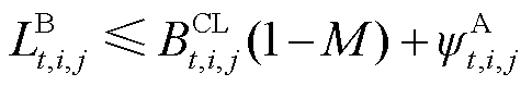
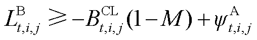
,反之 ;M为很大的正数,用于线性化模型;
 、
、 、
、 分别为0号柴油、92号汽油和95号汽油油品密度;
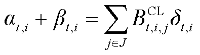
 为批次的油品种类指示标志,其取值见表1。经上述二进制转换,双线性项被等价重构为线性约束[26]。针对转换后约束中含有0-1变量与连续变量相乘的双线性项,可以利用后续3.1节中所提大M法进行进一步处理。
表1 辅助变量取值
Tab.1 Values of auxiliary variable

油品种类α 0号柴油000 92号汽油101 95号汽油112
针对压力损失中的油品体积分布和高程差难以定量表达的问题,本文将建模视角切换后上述问题得以解决。具体地,压力损失的计算从传统的直接计算每根管段内含有的批次油品的压力损失之和,切换到先计算所有批次油品的压力损失,再将其按长度和高程比例分配到不同管段中。综上所述,式(5)被等价重构为
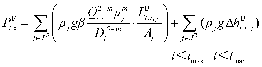 (16)
(16)
式中, 为所有批次集合;
 和
和 分别为第
分别为第 批次油品密度和粘度,其在批次视角下均为既定常数;
 和
和 分别为第个时间窗内第
![]() 批次油品在管段的水平长度和垂直高度,其显示表达为
批次油品在管段的水平长度和垂直高度,其显示表达为
 (17)
(17)
 (18)
(18)
 (19)
(19)
 (20)
(20)
 (21)
(21)
式中, 和
和 为引入的辅助连续变量,用于线性化模型;
 和
和 分别为管段的高程差和里程长度;
 为第个时间窗内第批次油头的体积位置坐标;
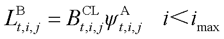
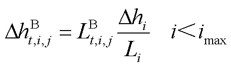
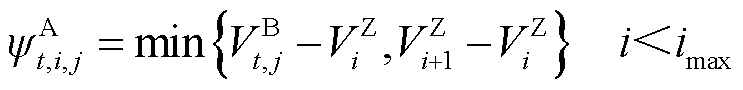
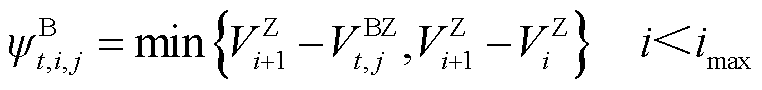
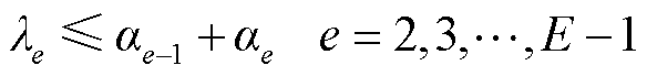
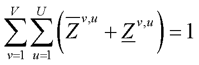
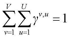
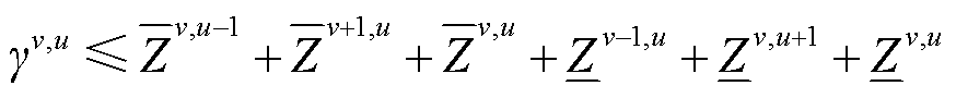
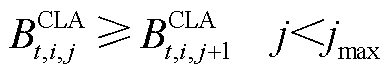
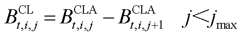
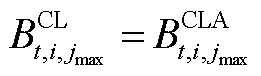
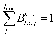
 为第个站场的体积位置坐标。式(19)的含义是利用管段的水平长度和高程差之比来近似油品的水平长度和高程差之比[27]。式(20)和式(21)是描述各批次油品在管段中的分布,其物理意义如图2所示,对于油品可能分布于管段首站、管段末站和贯穿管段的三种可能情况进行了数学描述,其中DS1、DS2和DS3分别为油品途径站场,不同序号代表不同油品。
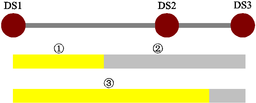
图2 油品分布示意图
Fig.2 Schematic diagram of refined oil distribution
本节在重构后模型的基础上,利用大M法、分段线性化和二维凸组合等线性化手段将模型进一步转换为易于求解的混合整数线性规划模型。
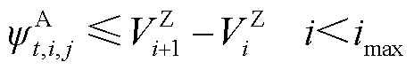
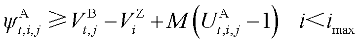
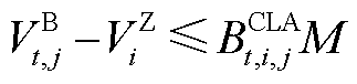
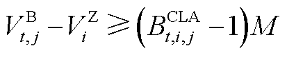
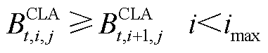
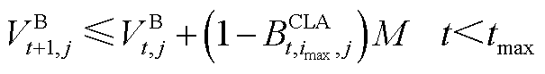
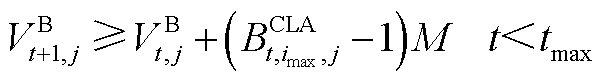
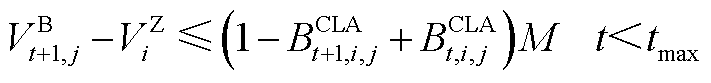
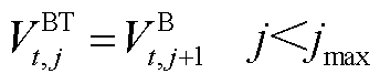
针对含min函数的约束式(20)和式(21),以式(20)为例利用大M法进行如下等价线性化,有
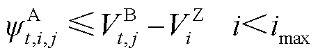 (22)
(22)
 (23)
(23)
 (24)
(24)
 (25)
(25)
式中, 和
和 为引入的0-1变量。
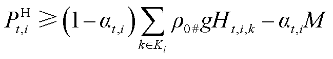
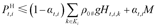
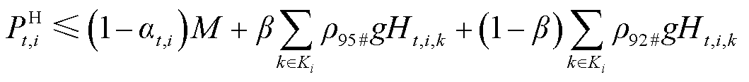
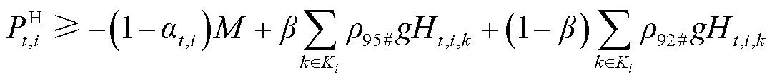
针对含有0-1变量和连续变量相乘项的约束式(11)~式(14)和式(17)、式(18),以式(17)为例进行等价线性化[28],有
 (26)
(26)
 (27)
(27)
 (28)
(28)
针对式(7)中扬程与流量的二次非线性关系和式(1)中电力成本与流量呈现的三次非线性关系,本文利用分段线性化技术对上述非线性项进行近似处理。
设与流量有关的函数表达式为 ,其中映射
,其中映射![]() 为函数的非线性关系。在给定的流量区间范围内,利用
为函数的非线性关系。在给定的流量区间范围内,利用![]() 个分段点,即
个分段点,即 ,将其分成
,将其分成 段,本文采取等分策略,将区间的分段点用
 ,
,  ,
,  ,
,  表示。其中与所给流量区间的下限重合,与所给流量区间的上限重合。每个分段点e均用一个连续变量
 进行关联,每个分段区间
 均用一个0-1变量
 进行关联,如图3所示。
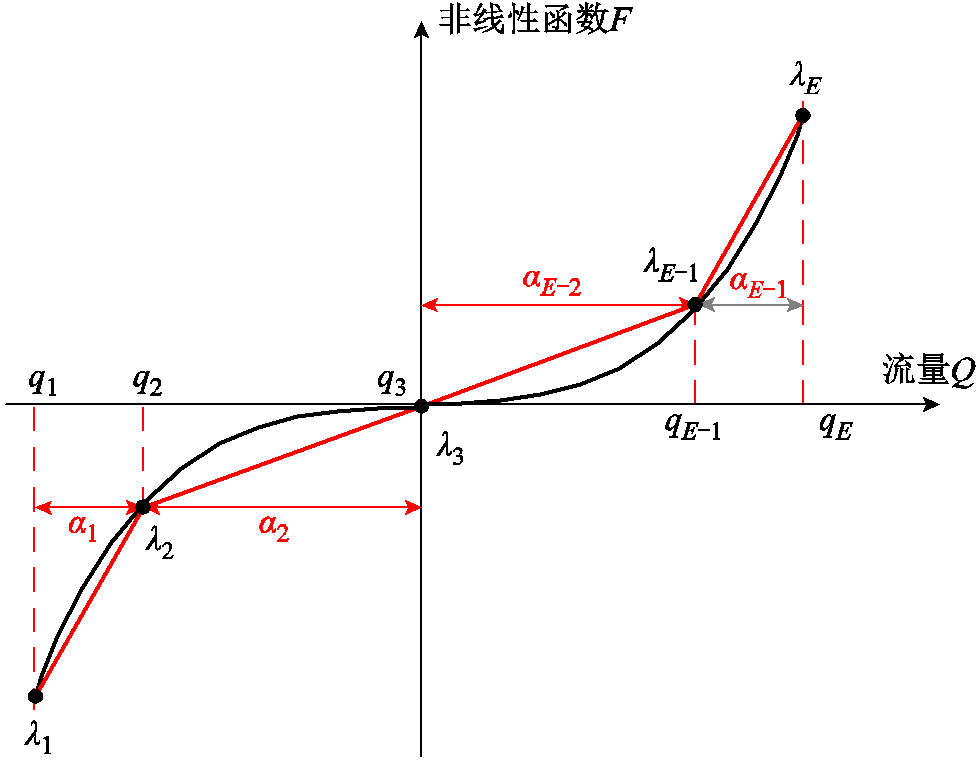
图3 分段线性化示意图
Fig.3 Schematic diagram of piecewise linearization
在给定的流量区间范围内,对于任意一个给定流量 ,及其对应函数的估计值
 都可以用式(29)~式(36)进行线性化表示[29]。
 (29)
(29)
 (30)
(30)
 (31)
(31)
 (32)
(32)
 (33)
(33)
 (34)
(34)
 (35)
(35)
 (36)
(36)
针对压力损失式(16)中存在的流量与批次体积相乘的双线性项,本文利用二维凸组合的方式对其进行线性化近似。
设二元函数表达式为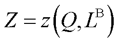 ,其中映射
,其中映射![]() 代表函数的非线性关系。根据文献[30],二维单纯形为三角形,因此本文在给定的流量区间范围内,利用V个分段点,即
代表函数的非线性关系。根据文献[30],二维单纯形为三角形,因此本文在给定的流量区间范围内,利用V个分段点,即 ,采取等分策略将流量区间分成V-1段,分段点用
 ,
,  , ,
, ,  表示。其中与所给流量区间的下限重合,与所给流量区间的上限重合;同样地,在给定的油品水平长度区间范围内,利用U个分段点,即
 采取等分策略将其分成U-1段,分段点用
 ,
,  , ,
, ,  表示,其中与所给长度区间的下限重合,与所给长度区间的上限重合。通过上述区间划分,可以将二元函数的曲面利用多个二维单纯形来近似替代。在函数定义域内,以由
 、
、 、
、 、
、 顶点构成的矩形为例,通过对角线分割,可以将矩形区域划分为上、下两个三角形,对应区域为上、下单纯形在
 平面的投影。
二维凸组合示意图如图4所示,每个分段点均采用一个连续变量 进行关联,每个上单纯形均用一个0-1变量
 ,
, 进行关联,每个下单纯形也用一个0-1变量
 进行关联。则对于函数定义域内任意一点
 的二元函数值,都可以利用其所在单纯形顶点的线性组合结果
 进行近似替代,如式(37)~式(43)所示。
 (37)
(37)
 (38)
(38)
 (39)
(39)
 (40)
(40)
 (41)
(41)
 (42)
(42)
 (43)
(43)
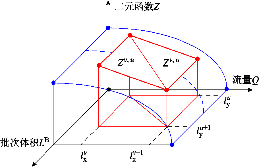
图4 二维凸组合示意图
Fig.4 Schematic diagram of 2D convex combination
本节在Matlab 2021a平台上以国内西南地区某成品油管线为算例对所提模型进行测试,测试环境为i7-7700 CPU@3.60 GHz,16 G内存,并调用商业求解器GUROBI 9.1.0进行求解。
算例管道长度约47.4 km,沿线共有五个站场,包括一个输油首站(即油品注入站IS)、三个中间下载站(即DS1、DS2和DS3)和一个输油末站(即TS),其中输油首站IS和中间下载站D1为泵站,决策总时长为24 h,线性化分段数均取5,其余算例参数见附表1~附表5。
1)基本求解结果
算例1:在本文所提模型得到的流量计划基础上,进一步利用文献[18]所提单一阶段优化模型求取压力分布和配泵方案。
算例2:在本文所提模型得到的流量计划基础上,进一步利用文献[20]所提两阶段联合优化模型求取压力分布和配泵方案。
算例3:本文所提两阶段联合优化模型。
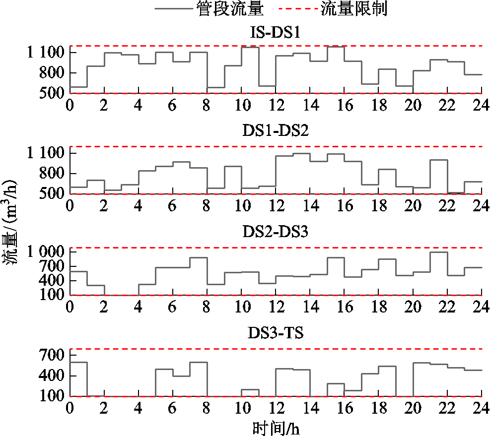
图5为求解所得批次转移图[31],从左至右用红、绿、蓝三种颜色分别代表0号柴油、92号汽油和95号汽油,左侧的纵轴代表计划初始时刻管段内只有0号柴油,矩形块的宽度代表成品油在各个时刻被各个站场所注入和下载的流量,流量越大矩形块越宽。此外,黑色斜线代表批次界面的移动,其中斜率的增大代表着对应管段流量的增大。图5中,已存在的0号柴油批次和待输送的三个批次均按时到达各个站场,且实时下载流量和累计下载流量分别满足下载安全限制和决策时段内总下游市场需求,表明所求流量计划的可行性,具体流量分布如附图1所示。
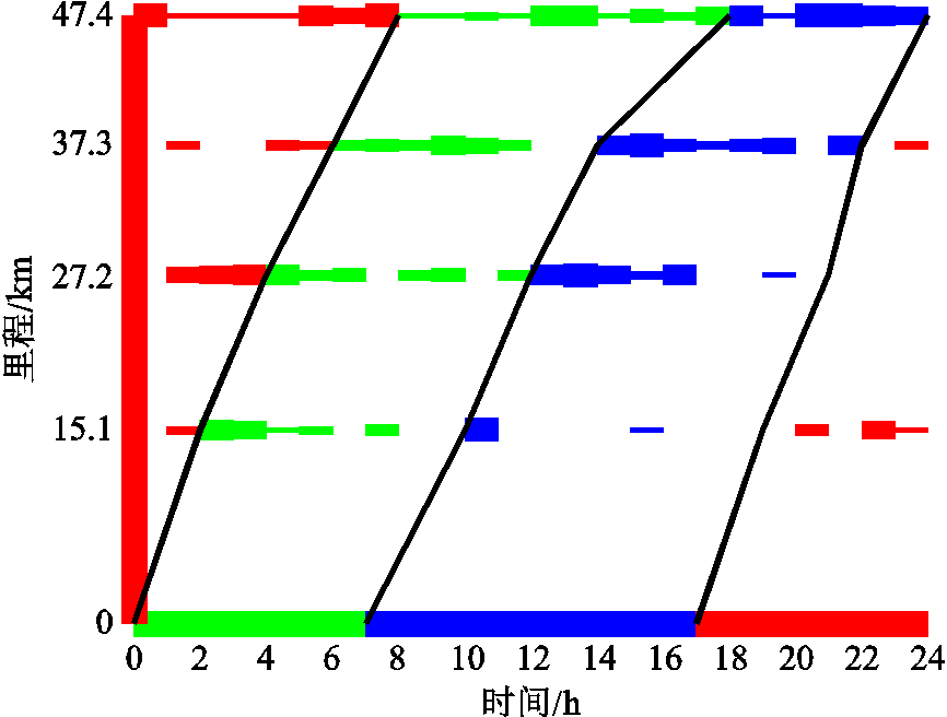
图5 算例1~3批次转移图
Fig.5 Batch moving plan in Case1 to Case 3
表2为相同流量计划下算例1~3求解结果,其中算例1为单一阶段优化模型,其求取结果为理论上最优解。因此本文将算例1求解结果定义为实际值,将近似误差定义为不同模型估计值与实际值的相对百分偏差。本文所提模型算例3在电力成本上比最优解仅高1.39%,而现有联合优化模型算例2的电力成本比最优解要高出27.95%,验证了所提模型的电力成本正确性。
表2 算例1~3求解结果对比
Tab.2 Result comparasion among Case1 to Case 3

对比指标算例1算例2算例3 电力成本/(103元)23.0429.4823.36 泵功率/(MW·h)27.1135.6027.49 泵提供压力/MPa112.97142.62112.99 压力损失/MPa105.97118.28105.36 泵站特性平均近似误差(%)—8.920.21 泵站特性最大近似误差(%)—10.510.41 压力损失平均近似误差(%)—19.740.61 压力损失最大近似误差(%)—42.171.80
上述差异源于不同模型对泵站特性和压力损失的近似误差不同,算例2对于两阶段模型中的非线性项采用常数替代连续变量,在简化计算过程的同时会导致所求结果过于保守。具体地,一方面,算例2对泵站特性的平均近似误差达10.51%,导致求解结果对电力成本进行了粗略的估计,难以反映实际泵能耗,可能导致不经济的配泵方案进而带来更高的电力成本;另一方面,算例2对压力损失的平均近似误差更是高达19.74%,难以反映实际成品油管网的压力工况,可能导致错误的配泵方案,进而危及运行安全。相比之下,算例3在泵站特性和压力损失的近似上都与实际值更为贴近,最大近似误差分别仅有0.41%和1.80%,验证了所提模型的近似精度。
图6为不同方案下的泵起停计划,其中黑色实心代表泵起动,空心代表泵停机。算例1和算例3所给配泵计划相同,从配泵角度验证了所提模型的正确性。相比之下,算例2由于对压力损失和泵站特性的近似过于保守,导致四台泵的总在线时长比算例3多出9 h,进一步恶化了经济性。值得注意的是,算例2在16 h给出了四台泵同时起动的方案,该方案意味着出现备用缺失的局面,一旦一台泵停机,将导致整条管线失去输送能力,造成巨大的经济损失。若给模型添加起泵数量约束,则会导致模型出现无解局面。因此,算例2所给开泵方案难以在实际调度中被采用。相比之下,本文所提模型能更准确地估计管网的压力损失,决策出更为合理的配泵方案。
图7为不同方案下的压力分布,算例3的压力分布平均近似误差仅为0.6%,验证了所提模型的压力分布正确性。相比之下,算例2由于对压力损失的近似误差较大,导致配泵方案出现冗余,进而导致管段压力分布贴近运行上限,甚至在压力损失较大的第1、9、11、16和22个时间窗内出现压力越限的局面。以10~11 h为例,不同方案的压力损失估计见表3。由于管段IS-DS1的流量较大,相较于其他管段其近似误差也较大。由于现有模型对压力损失的估计误差较大,高估了管段的压力损失,导致算例2不得不起动更多的泵来弥补估计误差,进而危及运行安全。
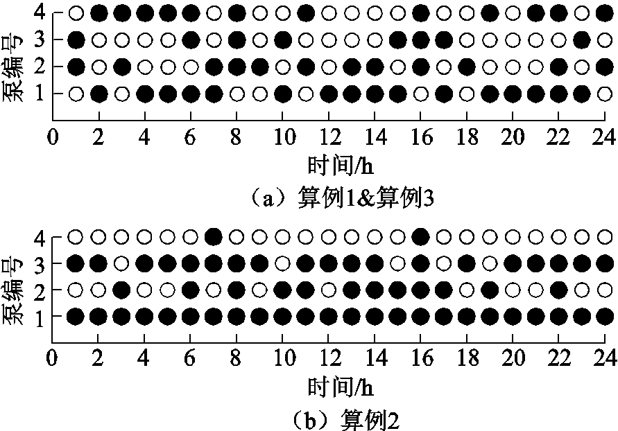
图6 算例1~3泵起停计划
Fig.6 Pump scheduling in Case 1 to Case 3
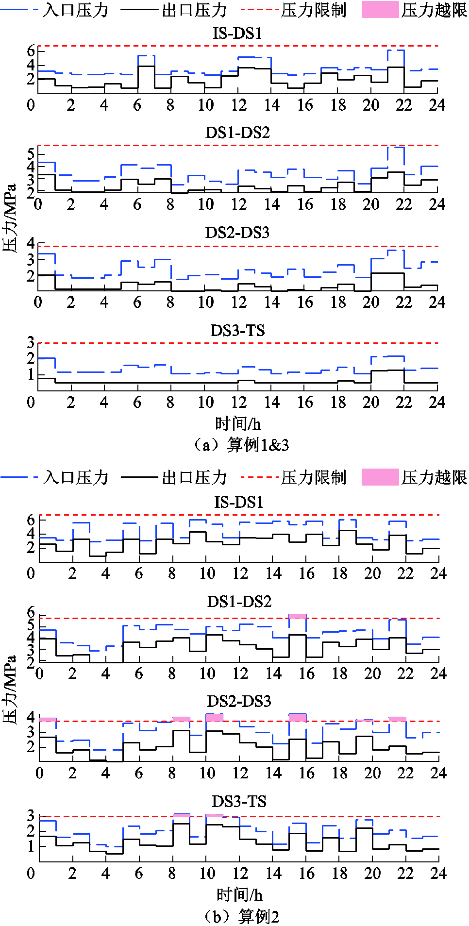
图7 算例1~3压力分布
Fig.7 Pressure distribution in Case1 to Case 3
表3 10~11 h压力损失估计
Tab.3 Pressure loss estimation in 10 h to 11 h (单位:MPa)

压力损失算例1算例2算例3 IS-DS11.802.551.80 DS1-DS20.700.830.71 DS2-DS30.941.090.95
2)分段数参数分析
本文所提模型在不同分段数下的计算结果见表4。当分段数少于3时,变量近似的最大误差高于10%,难以用于工程实际;当分段数大于5时,电力成本的降低不再显著,且由于引入了更多的整数变量使计算时间快速增长。可见,本文所提模型需要根据实际算例规模和模型求解时间来决策合理的分段数。
表4 不同分段数下的计算结果
Tab.4 Calculation results with different segment numbers
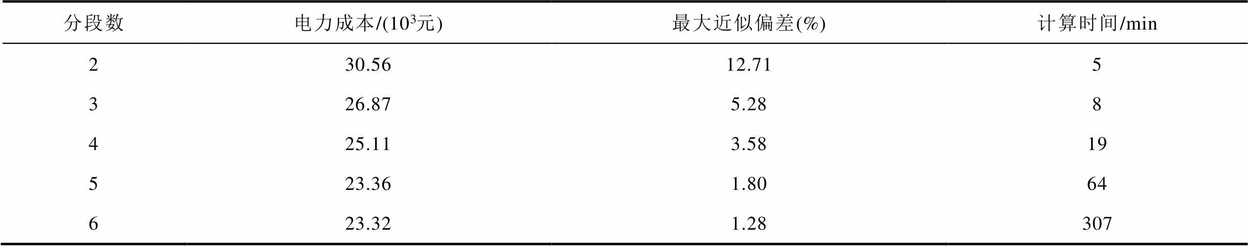
分段数电力成本/(103元)最大近似偏差(%)计算时间/min 230.5612.715 326.875.288 425.113.5819 523.361.8064 623.321.28307
本文基于批次视角和线性化技术建立了多批次成品油管网计划-运行联合优化模型,通过算例分析得到以下结论:
1)本文所提模型在近似精度上优于现有两阶段联合优化模型,且与单一阶段优化模型的最大近似误差仅有1.80%,验证了所提模型的有效性。
2)相较于现有联合优化模型,本文所提模型能够辨识出更经济且更安全的流量计划和配泵方案,电力成本降低27.95%,验证了所提模型的经济性。
3)本文分析了不同分段数下的求解结果,表明更多的分段数能够提高约束的近似精度,电力成本能进一步降低,但更多分段数也降低了模型的求解速度,因此需要根据实际算例规模和计算时间来决策分段数,确保模型求解时间和精度在合理范围内。
后续的研究可以进一步结合更多实际因素来完善本文所提模型,比如库存管理和动态电价等。
附 录
1. 联合优化模型流量约束
1)批次追踪约束
 (A1)
(A1)
 (A2)
(A2)
 (A3)
(A3)
 (A4)
(A4)
 (A5)
(A5)
 (A6)
(A6)
 (A7)
(A7)
 (A8)
(A8)
 (A9)
(A9)
式中, 为第
为第 个时间窗内第
![]() 批次油头的体积位置坐标;
批次油头的体积位置坐标; 为第
为第 个站场的体积位置坐标;
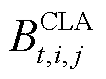 为第个时间窗内第
![]() 批次油头经过第个站场的状态变量,若油头已达到站场则
批次油头经过第个站场的状态变量,若油头已达到站场则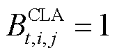 ,反之
,反之 ;
; 为第t个时间窗内第
![]() 批次油品在管段
批次油品在管段 内的状态变量,若该油品在管中,则
 ,反之
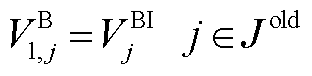
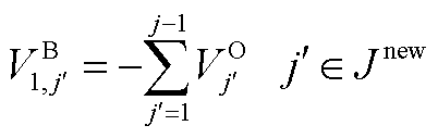
,反之 。式(A1)~式(A9)为批次过站约束,其本质是利用一维的数轴对各个批次的油头和油尾进行位置描述。式(A3)的含义是同一批次油品应按站场顺序依次过站。式(A4)的含义是不同批次油品应按批次顺序依次过站。式(A7)的含义是确保每根管段内始终含有成品油,即每个站场在任意个时间窗内均有一个批次过站。式(A9)的含义是每根管段内至多存在一个批次油头,即每根管段内至多存在两种不同成品油。
初始时间窗内批次位置约束为
 (A10)
(A10)
 (A11)
(A11)
式中, 为初始时刻管段内已有批次的初始体积坐标;
 为初始时刻尚未注入管段批次的油品体积;Jold为初始时间窗内管段所含油品批次集合。
批次油头坐标约束为
 (A12)
(A12)
 (A13)
(A13)
 (A14)
(A14)
 (A15)
(A15)
 (A16)
(A16)
 (A17)
(A17)
 (A18)
(A18)
式中, 为第t个时间窗内管段内油品流量。若批次油品已注入管段,则式(A12)和式(A13)即可更新油头位置;若批次尚未注入管段,则式(A14)和式(A15)即可更新油头位置;若批次油头已达终点站,则式(A16)和式(A17)即可更新油头位置;若油头恰好与站场坐标重合,则式(A18)即可更新油头位置。
批次油尾位置坐标描述为
 (A19)
(A19)
 (A20)
(A20)
 (A21)
(A21)
式中, 第t个时间窗内第
![]() 批次油尾的体积位置坐标。
批次油尾的体积位置坐标。
2)站场下载约束
 (A22)
(A22)
 (A23)
(A23)
 (A24)
(A24)
 (A25)
(A25)
式中, 为第t个时间窗内第j批次在第i个站场的下载流量;
 为第
为第![]() 批次油品对应第
批次油品对应第 个油品种类;
 为第i个站场在调度时段内所需第个油品种类的油品总体积;
 为第t个时间窗内第i个站场是否下载油品的状态变量,若下载则
![]() ,反之
,反之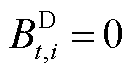 ;
; 和
和 分别为第i个站场下载油品的下载流量上、下限。式(A22)的含义是当且仅当批次油头过站且油尾未过站时才允许该站下载油品。
3)管段流量约束
 (A26)
(A26)
 (A27)
(A27)
 (A28)
(A28)
 (A29)
(A29)
式中, 为第t个时间窗内首站油品的注入流量;
 和
和 分别为管段内油品流量上、下限。式(A26)~式(A28)反映了成品油管网满足的质量守恒关系。
2. 算例系统参数及算例结果
附表1 站场下载参数
App.Tab.1 Delivery parameters of stations

站场0号需求/m392号需求/m395号需求/m3最小下载流量/(m3/h)最大下载流量/(m3/h) DS18501 100500100900 DS21 2001 4001 800100600 DS36801 4002 000100600 TS2 1001 8002 000100600
附表2 站场压力限制
App.Tab.2 Pressure limits of stations
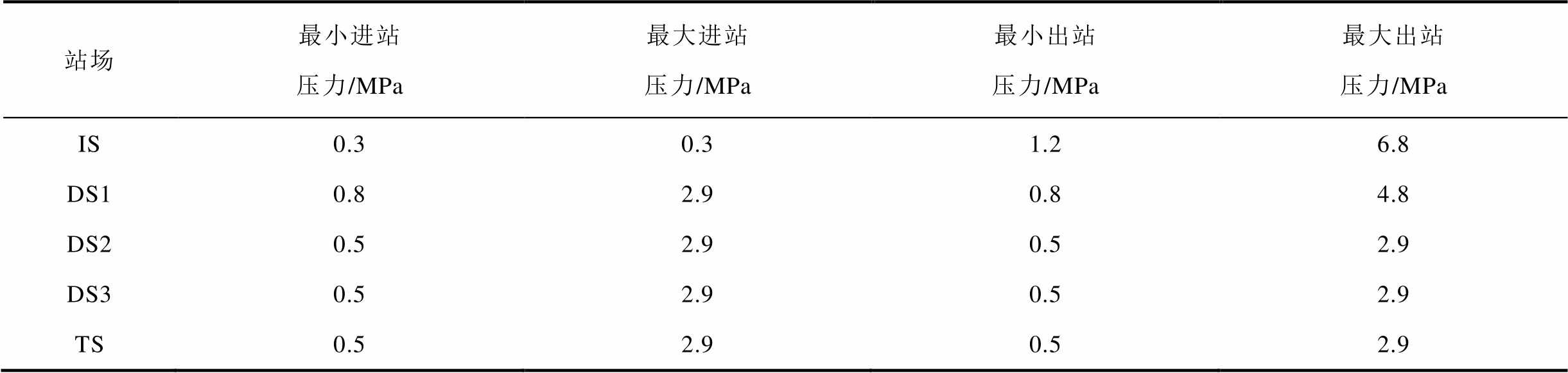
站场最小进站压力/MPa最大进站压力/MPa最小出站压力/MPa最大出站压力/MPa IS0.30.31.26.8 DS10.82.90.84.8 DS20.52.90.52.9 DS30.52.90.52.9 TS0.52.90.52.9
附表3 站场主输泵扬程参数
App.Tab.3 Pump head parameters of each pump

站场泵编号 IS(P1)P1-1-1.09-14.1497.1 P1-2-1.12-13.8498.2 DS1(P2)P2-1-44.9-5.6322.9 P2-2-43.2-5.8325.2
附表4 批次计划参数
App.Tab.4 Parameters of injection plan
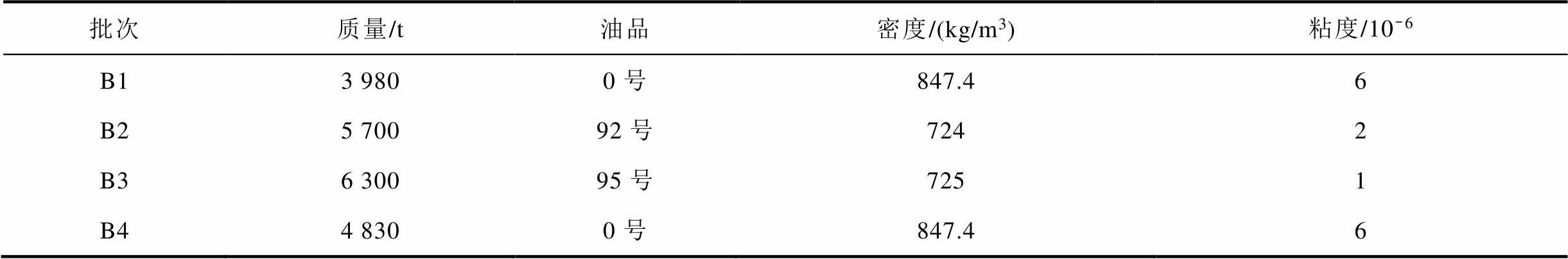
批次质量/t油品密度/(kg/m3)粘度/10-6 B13 9800号847.46 B25 70092号7242 B36 30095号7251 B44 8300号847.46
附表5 管段参数
App.Tab.5 Parameters of pipeline segments
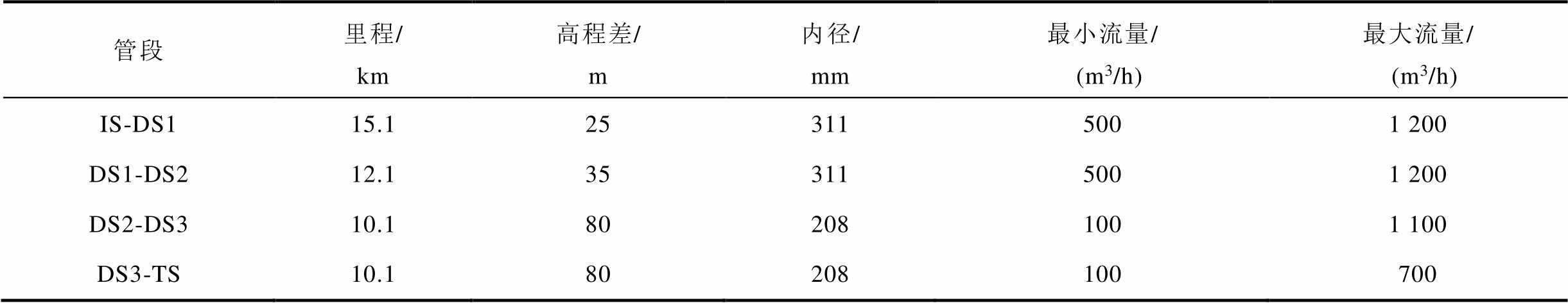
管段里程/ km高程差/ m内径/ mm最小流量/ (m3/h)最大流量/ (m3/h) IS-DS115.1253115001 200 DS1-DS212.1353115001 200 DS2-DS310.1802081001 100 DS3-TS10.180208100700
3. 算例结果图
附图1 算例1~3流量分布
App.Fig.1 Flow distribution in Case1 to Case 3
参考文献
[1] 胡泽春, 邵成成, 何方, 等. 电网与交通网耦合的设施规划与运行优化研究综述及展望[J]. 电力系统自动化, 2022, 46(12): 3-19. Hu Zechun, Shao Chengcheng, He Fang, et al. Review and prospect of research on facility planning and optimal operation for coupled power and transportation networks[J]. Automation of Electric Power Systems, 2022, 46(12): 3-19.
[2] 马伟明. 关于电工学科前沿技术发展的若干思考[J]. 电工技术学报, 2021, 36(22): 4627-4636. Ma Weiming. Thoughts on the development of frontier technology in electrical engineering[J]. Transactions of China Electrotechnical Society, 2021, 36(22): 4627-4636.
[3] 毛玲, 张钟浩, 赵晋斌, 等. 车-桩-网交融技术研究现状及展望[J]. 电工技术学报, 2022, 37(24): 6357-6371. Mao Ling, Zhang Zhonghao, Zhao Jinbin, et al. Research status and prospect of vehicle-pile-net blending technology[J]. Transactions of China Electrotechnical Society, 2022, 37(24): 6357-6371.
[4] Huang Weiqing, Wang Qiufang, Li Han, et al. Review of recent progress of emission trading policy in China[J]. Journal of Cleaner Production, 2022, 349: 131480.
[5] Wang Shengshi, Li Miao, Li Bin, et al. Optimal operation of integrated power and oil transmission systems[C]//2021 IEEE 4th International Electrical andEnergy Conference (CIEEC), Wuhan, China, 2021: 1-6.
[6] Zhou Xingyuan, Zhang Haoran, Qiu Rui, et al. A hybrid time MILP model for the pump scheduling of multi-product pipelines based on the rigorous description of the pipeline hydraulic loss changes[J]. Computers & Chemical Engineering, 2019, 121: 174-199.
[7] Zhou Xingyuan, Zhang Haoran, Xin Shengchao, et al. Future scenario of China’s downstream oil supply chain: low carbon-oriented optimization for the design of planned multi-product pipelines[J]. Journal of Cleaner Production, 2020, 244: 118866.
[8] Oikonomou K, Parvania M, Khatami R. Optimal demand response scheduling for water distribution systems[J]. IEEE Transactions on Industrial Informatics, 2018, 14(11): 5112-5122.
[9] Li Zhengbing, Liang Yongtu, Liao Qi, et al. A review of multiproduct pipeline scheduling: from bibliometric analysis to research framework and future research directions[J]. Journal of Pipeline Science and Engineering, 2021, 1(4): 395-406.
[10] Wang Shengshi, Zuo Lianyong, Li Miao, et al. The data-driven modeling of pressure loss in multi-batch refined oil pipelines with drag reducer using long short-term memory (LSTM) network[J]. Energies, 2021, 14(18): 5871.
[11] Zhou Xingyuan, Liang Yongtu, Zhang Xin, et al. A MILP model for the detailed scheduling of multiproduct pipelines with the hydraulic constraints rigorously considered[J]. Computers & Chemical Engineering, 2019, 130: 106543.
[12] Liao Qi, Castro Pedrom, Liang Yongtu, et al. New batch-centric model for detailed scheduling and inventory management of mesh pipeline networks[J]. Computers & Chemical Engineering, China, 2019, 130: 106568.
[13] Zuo Lianyong, Wang Shengshi, Ai Xiaomeng, et al. Sequential decision-making methods on real-time optimization of pump scheduling of refined oil pipelines[C]//2021 IEEE Sustainable Power and Energy Conference (iSPEC), Nanjing, 2021: 2177-2183.
[14] Losenkov A, Yushchenko T, Strelnikova S, et al. Optimization of oil-flow scheduling in branched pipeline systems[J]. Journal of Pipeline Systems Engineering and Practice, 2019, 10(3): 4019014.
[15] Haihong Chen, Lili Zuo, Changchun Wu, et al. Optimization on delivery schedules of a multiproduct pipeline based on the oil-demand mode[J]. Acta Petrolei Sinica, 2019, 40(8): 990.
[16] Hong Bingyuan, Li Xiaoping, Di Guojia, et al. An integrated MILP method for gathering pipeline networks considering hydraulic characteristics[J]. Chemical Engineering Research and Design, 2019, 152: 320-335.
[17] Xin Shengchao, Liang Yongtu, Zhou Xingyuan, et al. A two-stage strategy for the pump optimal scheduling of refined products pipelines[J]. Chemical Engineering Research and Design, 2019, 152: 1-19.
[18] Wang Shengshi, Fang Jiakun, Ai Xiaomeng, et al. Implementation and field test of optimal pump scheduling in the multiproduct refined oil transmissionsystem[J]. IEEE Transactions on Industry Applications, 2022, 58(6): 7930-7941.
[19] Chen Haihong, Zuo Lili, Wu Changchun, et al. Optimizing detailed schedules of a multiproduct pipeline by a monolithic MILP formulation[J]. Journal of Petroleum Science and Engineering, 2017, 159: 148-163.
[20] Liao Qi, Liang Yongtu, Xu Ning, et al. An MILP approach for detailed scheduling of multi-product pipeline in pressure control mode[J]. Chemical Engineering Research and Design, 2018, 136: 620-637.
[21] Liao Qi, Zhang Haoran, Xu Ning, et al. A MILP model based on flowrate database for detailed scheduling of a multi-product pipeline with multiple pump stations[J].Computers & Chemical Engineering, 2018, 117: 63-81.
[22] 赵汉中. 工程流体力学Ⅱ[M]. 武汉: 华中科技大学出版社, 2005.
[23] Mehanna O, Huang Kejun, Gopalakrishnan B, et al. Feasible point pursuit and successive approximation of non-convex QCQPs[EB/OL]. 2014: arXiv: 1410.2277. https://arxiv.org/abs/1410.2277.
[24] Cafaro V G, Cafaro D C, Méndez C A, et al. MINLP model for the detailed scheduling of refined products pipelines with flow rate dependent pumping costs[J]. Computers & Chemical Engineering, 2015, 72: 210-221.
[25] Zabihi R, Mowla D, Karami H R. Artificial intelligence approach to predict drag reduction in crude oil pipelines[J]. Journal of Petroleum Science and Engineering, 2019, 178: 586-593.
[26] 张谦, 邓小松, 岳焕展, 等. 计及电池寿命损耗的电动汽车参与能量-调频市场协同优化策略[J]. 电工技术学报, 2022, 37(1): 72-81. Zhang Qian, Deng Xiaosong, Yue Huanzhan, et al. Coordinated optimization strategy of electric vehicle cluster participating in energy and frequency regulation markets considering battery lifetime degradation[J]. Transactions of China Electrotechnical Society, 2022, 37(1): 72-81.
[27] Chen Lei, Yuan Ziyun, Xu Jianxin, et al. A novel predictive model of mixed oil length of products pipeline driven by traditional model and data[J]. Journal of Petroleum Science and Engineering, 2021, 205: 108787.
[28] 姜云鹏, 任洲洋, 李秋燕, 等. 考虑多灵活性资源协调调度的配电网新能源消纳策略[J]. 电工技术学报, 2022, 37(7): 1820-1835. Jiang Yunpeng, Ren Zhouyang, Li Qiuyan, et al. An accommodation strategy for renewable energy in distribution network considering coordinated dispatching of multi-flexible resources[J]. Transactions of China Electrotechnical Society, 2022, 37(7): 1820-1835.
[29] 徐玉琴, 方楠. 基于分段线性化与改进二阶锥松弛的电-气互联系统多目标优化调度[J]. 电工技术学报, 2022, 37(11): 2800-2812. Xu Yuqin, Fang Nan. Multi objective optimal scheduling of integrated electricity-gas system based on piecewise linearization and improved second order cone relaxation[J]. Transactions of China Electrote-chnical Society, 2022, 37(11): 2800-2812.
[30] Marco B. Solving mixed-integer programming problems using piecewise linearization methods[D]. Konstanz: Universität Konstanz, 2017.
[31] Yu Li, Wang Sujing, Xu Qiang. Optimal scheduling for simultaneous refinery manufacturing and multi oil-product pipeline distribution[J]. Computers & Chemical Engineering, 2022, 157: 107613.
Abstract Unlike water pipeline networks that transport a single medium, refined oil pipeline networks transport multiple media sequentially. As a result, the pipeline network parameters continuously vary over time, leading to multiple continuous time-varying variable multiplication terms in pressure constraints that exhibit strong nonlinearity. Existing research typically divides the transport of refined oil into two separate decision stages or simplifies the constraints to reduce model nonlinearity. However, most methods suffer from low safety or poor economics. To address these issues, this paper proposes a joint scheduling and operation optimization model for multi-batch refined oil pipeline network based on pressure constraint reconstruction. The model's accuracy is improved through model reconstruction and linear approximation, which accurately reflects the complex transportation conditions of refined oil pipeline networks.
First, according to different approaches to describe fluid motion in fluid mechanics, the construction of refined oil transport models switches from the traditional Eulerian-based network perspective to the Lagrangian-based batch perspective. Without compromising model accuracy, continuous time-varying variables in pressure constraints are reconstructed equivalently as discrete variables to reduce model nonlinearity. Simultaneously, some difficult-to-quantify variables are equivalently reconstructed as new variables that are easy to express and have intuitive physical meanings. Various linearization techniques, such as the big-M method, piecewise linearization and two-dimensional convex combination, are further utilized to eliminate the nonlinearity of the reconstructed model. Within the acceptable range of practical engineering errors, the two-stage joint optimization model is transformed into a tractable mixed integer linear programming model.
The proposed model is applied to a refined oil transportation pipeline network in the southwest region of China. Compared with the pump scheduling of existing models, the electricity cost of the proposed model is only 1.39% higher than the optimal solution. On the other hand, the electricity cost of the existing joint optimization model is 27.95% higher than the optimal solution. These results validate the power cost accuracy of the proposed model. Furthermore, pump station characteristics and pressure loss in the proposed model are closer to the actual values, with maximum approximation errors of only 0.41% and 1.80%, respectively. This validates the model's approximation accuracy. In contrast, the maximum approximation error of existing models reaches 19.74%, making it difficult to reflect the actual pressure conditions of refined oil pipeline networks. This can lead to incorrect pump allocation schemes, which worsens both economic efficiency and operational safety. Simulation results show that the pumping scheduling provided by the existing model could not be used in the implement field.
The simulation analysis leads to the following conclusions: (1) The proposed model has superior approximation accuracy compared to existing two-stage joint optimization models, which reflects the complex conditions of refined oil pipeline networks more accurately. (2) The proposed model can determine more accurate pump allocation schemes compared to existing models, which ensures transportation safety and improves economic efficiency. (3) A larger number of segments can improve the approximation accuracy of the constraints, which further reduces electricity costs. However, this comes at the cost of model solution speed. Therefore, the number of segments should be selected based on the actual model size and computation time.
keywords:Multi-batch transportation, linearization technique, electricity costs, energy saving in oil transportation
DOI:10.19595/j.cnki.1000-6753.tces.L10067
中图分类号:TM727
国家自然科学基金项目(52177089)和国家管网科技攻关项目(GWHT20200001399)资助。
收稿日期 2023-01-13
改稿日期 2023-03-29
刘晶冠 男,1999年生,硕士研究生,研究方向为综合能源系统优化建模。E-mail:spencerplusmail@foxmail.com
方家琨 男,1985年生,教授,博士生导师,研究方向为氢能、储能技术的系统应用、综合能源系统优化建模等。E-mail:jfa@hust.edu.cn(通信作者)
(编辑 赫蕾)