 为正定矩阵;P<0表示为负定矩阵;*表示对称矩阵中的对称项;In×n、0n×n分别为n×n单位矩阵和n×n零矩阵;diag(·)表示对角矩阵;ei (i=1, 2,…)表示分块单位矩阵;Sym(X)=XT+X。
摘要 该文研究了具有时变时滞和负荷扰动的负荷频率控制系统的稳定性问题。首先,构造新的增广向量和具有多重积分项的Lyapunov-Krasovskii泛函,建立不同变量间的耦合关系;其次,为了与所构造的泛函紧密配合,提出基于时滞相关矩阵和自由矩阵的积分不等式及基于时滞相关矩阵的反凸组合不等式,对泛函导数进行更精确的估计,从而得到具有较小保守性的负荷频率控制系统的稳定性判据;最后,通过对典型二阶时滞系统和单区域时滞负荷频率控制系统进行仿真分析,验证了所得的稳定性判据具有较小保守性,并分析了负荷扰动和控制器参数对系统时滞上界的影响。
关键词:电力系统稳定性 负荷频率控制 时变时滞 Lyapunov-Krasovskii泛函 时滞相关矩阵
频率是衡量电能质量的关键指标之一,频率稳定性对电力系统稳定运行至关重要[1]。频率的波动可能会使发电机和辅机偏离运行状态,从而给电力系统稳定运行及用户正常用电造成不利影响,所以电网频率需维持在某个固定值或在其附近小范围内上下浮动,而负荷频率控制(Load Frequency Control, LFC)是实现这一目标的有效方法之一,在维持电网频率和不同区域间的联络线功率交换方面发挥着重要作用[2-5]。目前,LFC在广域互联电力系统中得到了广泛应用。
LFC系统中数据测量、信号传输等大多需借助开放式通信网络,这种开放式通信网络可有效地降低成本且可实现大范围、大数据量的信息交换[6-7]。在借助通信网络构成信号传输、控制回路时,由于网络带宽的限制,在传输中不可避免地存在通信时滞、数据丢失、网络阻塞与攻击等问题。其中时滞问题普遍且突出,该问题的存在可能会导致电力系统动态性能恶化甚至不稳定[8-9]。因此,考虑时滞影响下LFC系统的稳定性问题具有重要的理论和现实意义,已成为诸多学者关注的焦点。
目前,研究时滞系统稳定性问题的主要方法有频域法和时域法。频域法主要基于特征根的分布来判断系统的稳定性,但往往需要通过求解超越方程得到特征根,计算过程复杂且存在难以求解的问题,因此该方法具有一定的局限性。相比于频域法,时域法能够较好地处理系统运行时状态信息发生跳变的情况,且计算过程更加简便,目前已成为分析时滞LFC系统稳定性的主要方法。时域法中应用最为广泛的是Lyapunov-Krasovskii(L-K)泛函方法[10]。由于此方法给出的是系统稳定的充分条件,必然存在一定的保守性。为了降低结果的保守性,诸多学者在L-K泛函构造和泛函导数估计两个方面进行了深入研究,一些新的L-K泛函构造方法和新的积分不等式被不断地提出。如泛函构造时有时滞分割方法[11]、增广型L-K泛函[12]、多重积分项L-K泛函[13]、Delay-product型L-K泛函[14]等方法;在泛函导数估计时有Jensen不等式[15]、基于Wirtinger积分不等式[9]、基于Free-matrix积分不等式[16]、Relaxed积分不等式[17]、基于Auxiliary-function积分不等式[18]、Bessel-Legendre积分不等式[19]及不同形式的反凸组合不等式[20]等。文献[5]通过建立一个增广型L-K泛函,并利用Bessel-Legendre积分不等式对导数进行处理,给出了LFC系统的最大时滞上界。文献[6]针对双时滞微电网,构造了一个具有更多增广项的L-K泛函,然后应用基于辅助函数的积分不等式,得到了微电网LFC系统的稳定性判据。文献[9]讨论了受数据采样时滞影响的LFC系统稳定性,为充分利用基于Wirtinger积分不等式,构造了与积分不等式紧密配合的增广型L-K泛函,从而得到了保守性较小的稳定性判据。文献[18]通过构造含有三重积分项的增广型L-K泛函,并应用基于Intermediate-auxiliary-function二重积分不等式对泛函导数进行估计,得到了更精确的估计边界,从而获得了时滞LFC系统保守性更小的稳定性判据。文献[21]通过增广向量,得到增广型L-K泛函,然后结合基于无穷级数的积分不等式,得到了时滞LFC系统稳定性判据。文献[22]通过提出一种基于低阶时滞相关的L-K泛函,并应用基于Wirtinger积分不等式对其导数进行估计,获得了LFC系统较大的时滞上界。需要注意的是,上述文献采用的方法虽然对获得较小保守性的稳定性判据有较大贡献,但在L-K泛函构造方法、泛函导数估计及两者有效配合上仍存在较大的提升空间。
基于上述讨论,本文进一步研究具有时滞影响和负荷扰动的LFC系统稳定性问题,目的是得到保守性更小的稳定性判据,并深入分析控制器参数对系统时滞上界的影响。首先,充分考虑系统时滞及其导数信息,构造一个包含新的增广向量和多重积分项的L-K泛函,以建立不同变量间的耦合关系,有助于降低稳定性判据的保守性。其次,为了更精确地估计泛函导数,提出基于时滞相关矩阵(Delay-Dependent-Matrix-Based, DDMB)和基于自由矩阵(Free-Matrix-Based, FMB)的积分不等式,该不等式与所构造的L-K泛函进行有效配合,能更精确地估计泛函导数。与现有的基于常数矩阵的积分不等式估计方法相比,这种新的积分不等式通过引入时滞相关矩阵,能充分利用更多的时滞信息。再次,提出扩展的基于时滞相关矩阵(Extended Delay-Dependent-Matrix-Based, EDDMB)的反凸组合不等式,突破现有反凸组合不等式的局限性,扩大其适用范围。此外,还使用基于辅助函数的积分不等式,从而得到较小保守性的稳定性判据。最后,通过对典型的二阶时滞系统和单区域时滞LFC系统仿真,验证了本文方法的有效性。
文中符号说明:Rn为n维欧几里德空间;P>0表示为正定矩阵;P<0表示为负定矩阵;*表示对称矩阵中的对称项;In×n、0n×n分别为n×n单位矩阵和n×n零矩阵;diag(·)表示对角矩阵;ei (i=1, 2,…)表示分块单位矩阵;Sym(X)=XT+X。
LFC系统模型主要包括发电机-负荷、原动机、调速系统、辅助LFC控制器等模型。发电机-负荷模型主要描述发电机输入端的机械功率变化、电网负荷变化及相应频率偏离量之间的相互关系。原动机主要用于产生机械功率进而带动发电机组发电,一次调频也依靠原动机来完成。原动机可以分为许多类别,如水轮机、汽轮机、燃气轮机等,为了便于分析且不失一般性,本文原动机模型选用常用的非再热式汽轮机。调速系统主要用于系统一次调频;辅助LFC控制器主要通过辅助控制器进行系统二次调频。在电力系统的分析和控制中,往往根据不同的控制问题和目标建立不同的模型。相对于电网电压和功角等快速动态过程,频率响应属于较慢的动态过程,在针对负荷端扰动的分析和设计时,往往采用简化的低阶线性系统来表征系统在运行点附近的动态特征。因此,在对系统建模时,只需用简化模型表示出各部分与频率相关的主要特性即可。
考虑时滞影响和负荷扰动的负荷频率控制系统模型结构如图1所示。
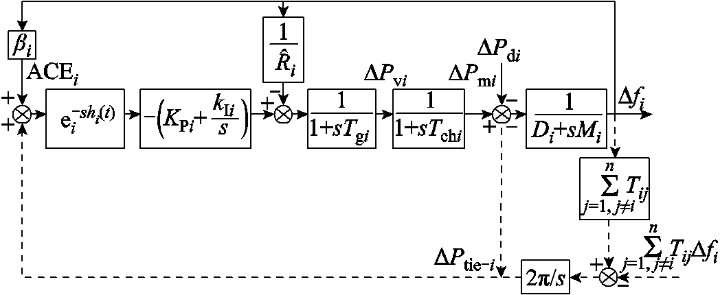
图1 考虑时滞和负荷扰动的LFC结构框图
Fig.1 Block diagram of LFC structure with time delay and load disturbance
其状态空间模型可表示为
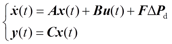 (1)
(1)
其中
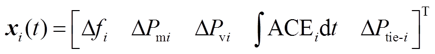
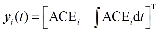
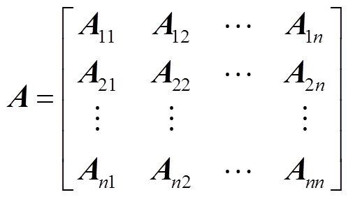
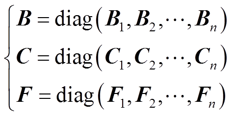
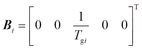
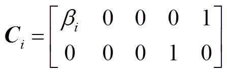
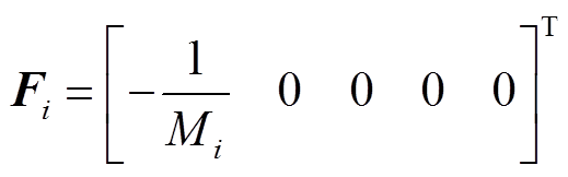
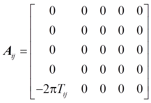
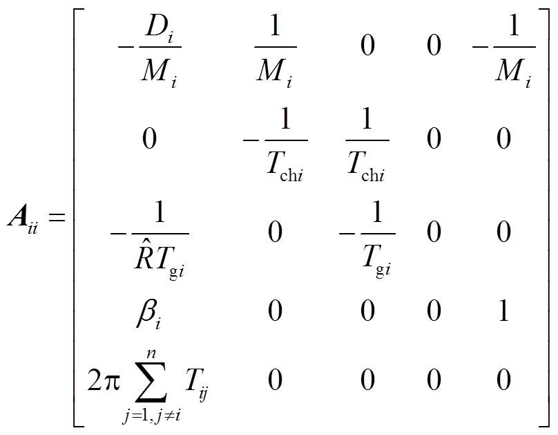
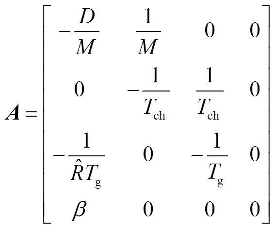
式中,A、B、C、F为系统矩阵;x(t)为系统状态变量;u(t)为控制输入;y(t)为测量输出;i和j为控制区域编号,i, j= 1, 2,…, n;n为电力系统中控制区域总数;Tij为区域i和区域j的联络线同步系数,Tij=Tji;ΔPtie-i为区域 联络线上的净交换功率偏差。假设每个控制区域的发电单元都相同,对于某个控制区域,Δf为系统频率变化量;ΔPm为机械功率变化量;ΔPv为汽门控制阀开度变化量;ΔPd为电网负荷变化量;M为发电机转动惯量;D为发电机阻尼系数;Tch为汽轮机惯性时间常数;Tg为调速器惯性时间常数;ACE为区域控制误差(area control error);
 为调速器的速度跌落系数;β为频率偏差因子。频率调节的基本原理为:当电网负荷变化ΔPd导致系统频率产生偏差Δf,该频率偏差产生一个调节原动机的反馈信号ΔPv,使原动机的输出功率增量ΔPm补偿负荷的变化量,从而使系统频率回到给定值。广域电力系统通常可分为多个区域,多区域LFC系统增加了连接各区域间的联络线,各区域间需要进行功率交换,因此多区域LFC系统控制目标不仅要控制本区域的频率为设定值,还需要控制区域间的功率交换为设定值。
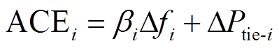
区域控制误差(ACE)通常采用区域频率偏差与联络线功率控制模式。第i个区域控制误差定义为
 (2)
(2)
其中,βi>0。将 作为第个控制器的输入,可以得到PI控制器为
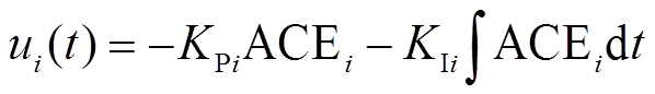 (3)
(3)
式中,KPi和KIi分别为第个控制器的比例和积分增益。
如图1所示,从到PI控制器的通信时滞用指数函数 来表示。故在考虑时滞影响情况下,式(3)可转换为
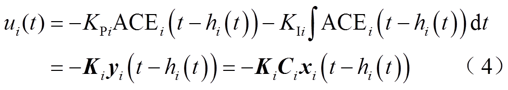
式中,hi(t)为第个区域的时变时滞;Ki=[KPi KIi]。
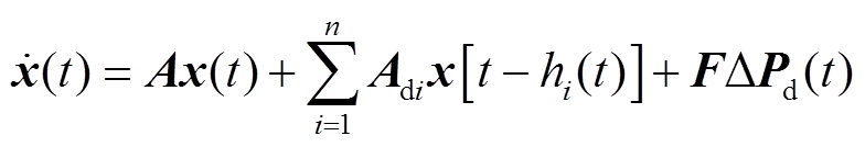
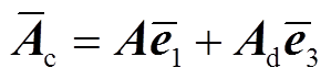
综合式(1)~式(4),可得具有时变时滞的LFC闭环系统动态模型为
 (5)
(5)
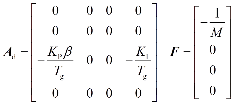
其中
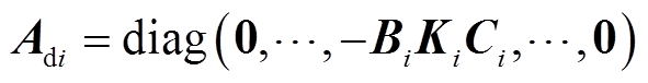
式中,Adi亦为系统矩阵。
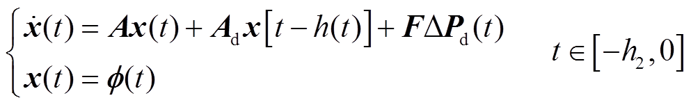
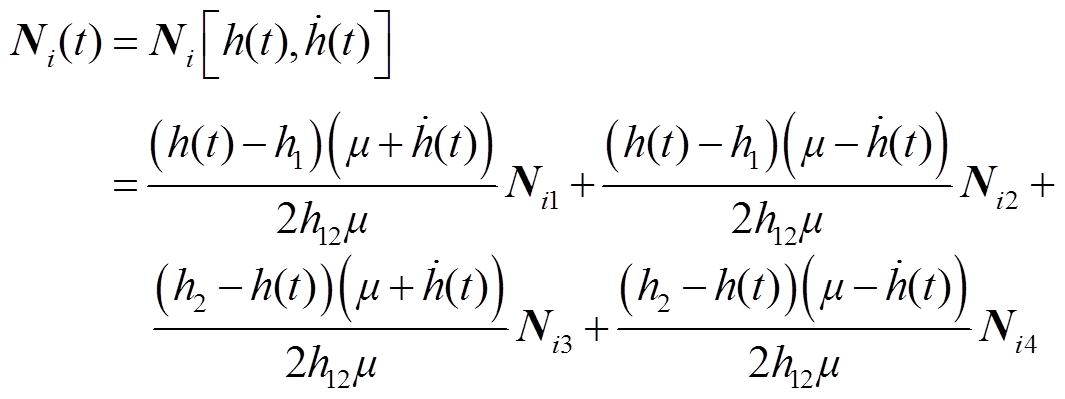
为方便分析,假设各区域时滞均相同,即h1(t)= h2(t)=…= hi(t)= hn(t)= h(t)。令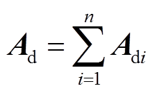 ,则具有时变时滞的LFC闭环系统动态模型可进一步简化为
 (6)
(6)
式中, 为系统初始状态;h2为时滞上界,为常数;h(t)为时变时滞,满足
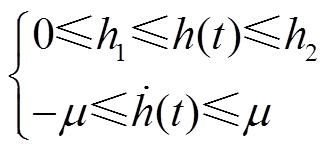 (7)
(7)
式中,h1和μ为常数,h1为时滞下界,μ<1。
为了估计负荷扰动对电力系统的影响,未知的负荷扰动可以假设为当前状态和时滞状态变量的非线性扰动[5,18],即
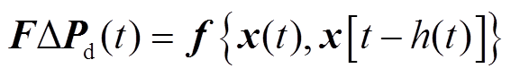 (8)
(8)
且满足条件
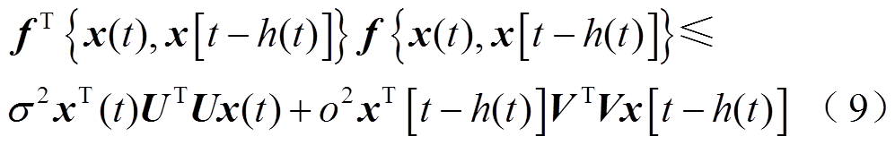
式中,U、V为适维的常数矩阵;σ、o为已知的非负标量。
特别地,当 ,即系统为单区域LFC时,有
本文的主要结论需用到以下命题和引理。
命题1:(DDMB和FMB积分不等式)若对于给定的对称矩阵 、
、 ,可微函数
,可微函数 ,以及任意矩阵
 和
和 满足
满足
则有
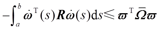 (10)
(10)
其中
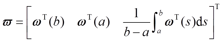
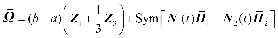
式中, 为任意常数矩阵。
证明:定义
 ,
,
因 ,故
,故 。结合如下积分等式:
 ,
,  ,
,
 ,
,  ,对函数
,对函数 从a到b积分,可得到
 (11)
(11)
由此,可以得到
证毕。
需要注意的是,本文提出了命题1,与传统的自由矩阵(FMB)积分不等式(文献[16]中的引理4)不同,该命题包含了时滞相关矩阵 , i=1, 2,引入了更多的自由矩阵,并充分利用了时滞
 及其导数
及其导数 信息,为有效降低结果的保守性提供了更大空间。当
 , i=1, 2时,命题1可简化为传统的FMB积分不等式,从而更具一般性。
命题2:(EDDMB反凸组合不等式)令 ,
, ,
, 及标量
及标量 ,如果存在时变时滞
 和时滞相关矩阵
 使得
使得
则有
其中
式中, 为任意常数矩阵。
需要注意的是,相比于现有的时滞相关矩阵(DDMB)反凸组合不等式(文献[20]引理2),命题2放松了对时滞下界h1=0的限制,h1可以取大于等于0的不同值。当h1=0时,命题2简化为DDMB反凸组合不等式。因此命题2更具一般性。
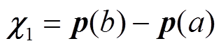
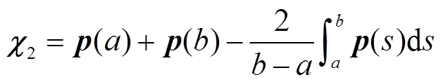
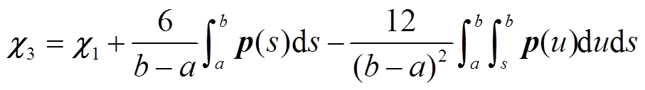
引理1[17]:对于对称矩阵R>0,实标量 、
、 ,且a<b,以及可微函数
 ,则积分不等式(13)成立,即
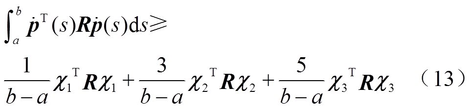
其中
引理2[18]:对于对称矩阵Q>0,可微函数 ,则积分不等式(14)、式(15)成立。
 (14)
(14)
 (15)
(15)
其中
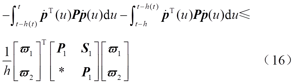
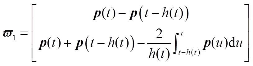
引理3[17]:对于对称矩阵 且满足P>0,实标量h>0,可微函数
 ,以及任意适维矩阵
 满足
满足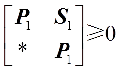 ,则积分不等式(16)成立。
其中
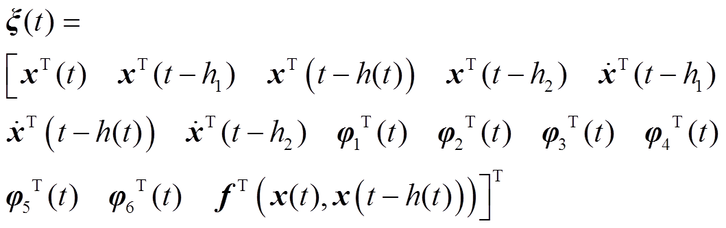
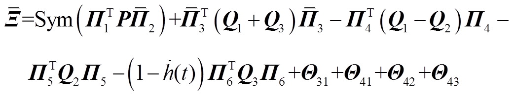
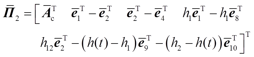
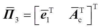
本节通过构造一个合适的L-K泛函,并采用新的分析方法,得到具有较小保守性的稳定性判据。为简化表述,定义如下向量。

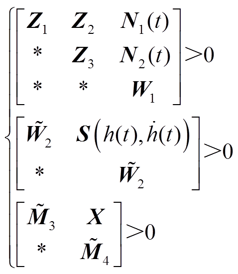
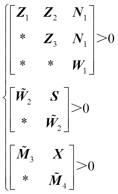
定理1:对于给定标量0≤h1≤h2,μ<1和λ>0,若存在对称正定矩阵 、
、 、
、 、
、 ,以及对称矩阵
 、
、 、
、 、
、 ,对于任意
,对于任意 、
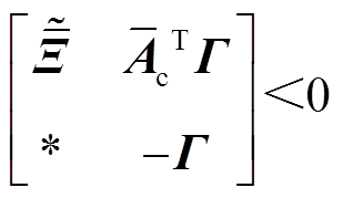
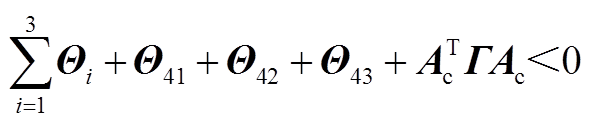
、 ,使得矩阵不等式(17)和式(18)成立,则系统式(6)渐近稳定。
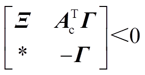 (17)
(17)
 (18)
(18)
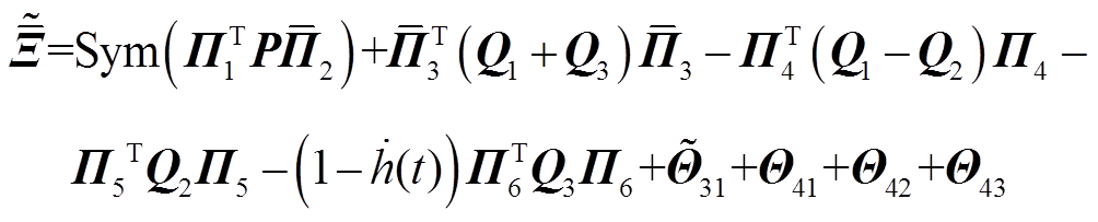
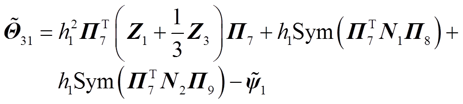
其中


证明过程详见附录。
当LFC系统无负荷扰动时,只需使系统式(6)中的 ,则
,则 。在定理1的基础上可得推论1。
推论1:在系统无负荷扰动情况下,即时,对于给定标量0≤h1≤h2、μ<1,若存在对称正定矩阵、、、,以及对称矩阵、、、,对于任意、,使得矩阵不等式(19)和式(20)成立,则系统式(6)在无负荷扰动时渐近稳定。
 (19)
(19)
 (20)
(20)
其中

式中, 如定理1中所示。
为了说明本文提出的DDMB和FMB积分不等式、EDDMB反凸组合不等式在估计泛函导数时的优势,在推论2中采用传统的FMB积分不等式和反凸组合不等式对L-K泛函的导数进行估计。
推论2:在系统无负荷扰动情况下,即时,对于给定标量0≤h1≤h2、μ<1,若存在对称正定矩阵、、、,以及对称矩阵、 、
、 、
、 ,对于任意、,使得矩阵不等式(21)和式(22)成立,则系统式(6)在无负荷扰动时渐近稳定。
 (21)
(21)
 (22)
(22)
其中
其余符号的定义见推论1。
本节通过对典型的二阶时滞系统和单区域时滞LFC系统进行仿真分析,说明本文结论的优越性;同时,还分析了单区域时滞LFC系统在不同条件下控制器参数对时滞上界的影响。
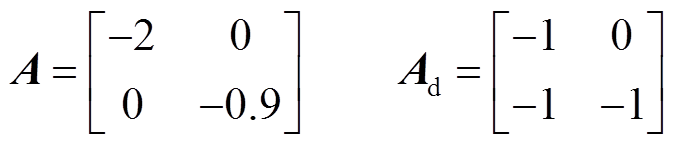
考虑时滞系统式(6)中时,即不考虑负荷扰动情况,系统参数为
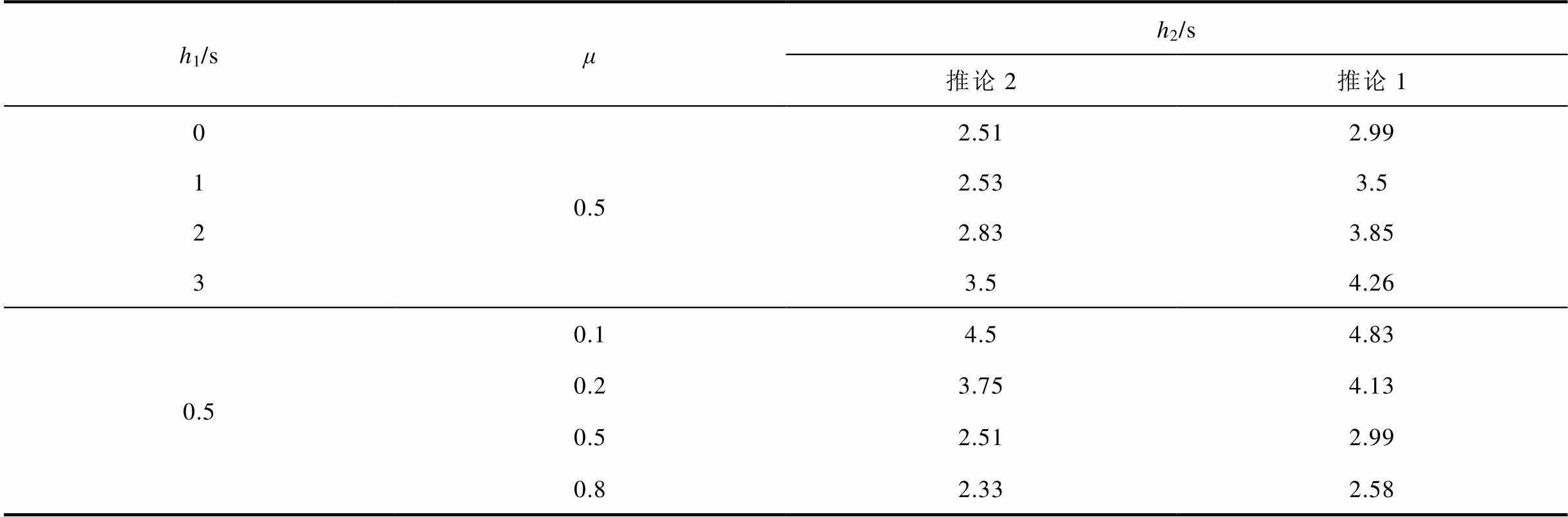
推论1和推论2在时滞下界h1、时滞变化率μ取不同值时所得到的时滞上界h2见表1。可以看出,当μ=0.5、h1=2s时,推论1得到的时滞上界h2比推论2提高了36.04%;当μ=0.5、h1=0时,推论1得到的时滞上界h2比推论2提高了19.12%。因此,应用本文提出的积分不等式能有效提高时滞上界,扩大稳定裕度。
表1 推论1与推论2结果对比
Tab.1 Comparative results of Corollary 1 and Corollary 2
h1/sμh2/s 推论2推论1 00.52.512.99 12.533.5 22.833.85 33.54.26 0.50.14.54.83 0.23.754.13 0.52.512.99 0.82.332.58
表2、表3列出了本文推论1与现有部分文献得到的时滞上界对比数据。
表2 h1取不同值、µ=0.5时,时滞上界h2结果对比
Tab.2 Comparative results of h2 for given h1 with µ=0.5(单位:s)
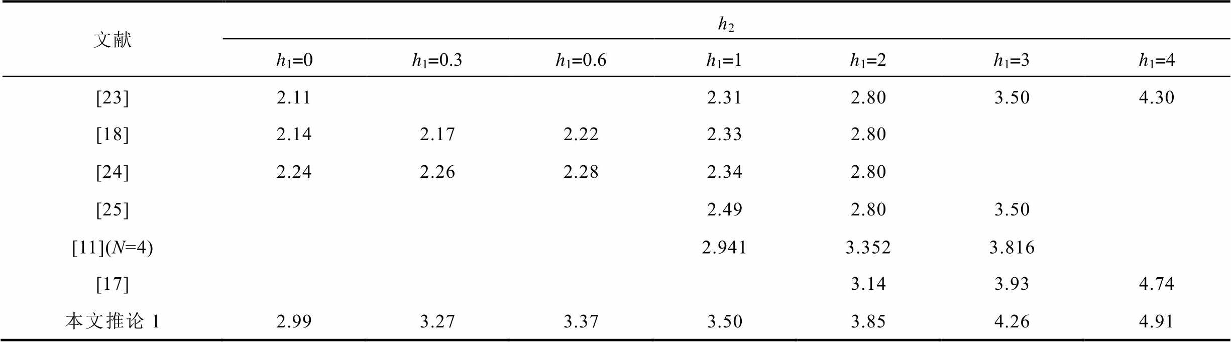
文献h2 h1=0h1=0.3h1=0.6h1=1h1=2h1=3h1=4 [23]2.112.312.803.504.30 [18]2.142.172.222.332.80 [24]2.242.262.282.342.80 [25]2.492.803.50 [11](N=4)2.9413.3523.816 [17]3.143.934.74 本文推论12.993.273.373.503.854.264.91
表3 µ取不同值、h1=0时,时滞上界h2结果对比
Tab.3 Comparative results of h2 for given µ with h1=0
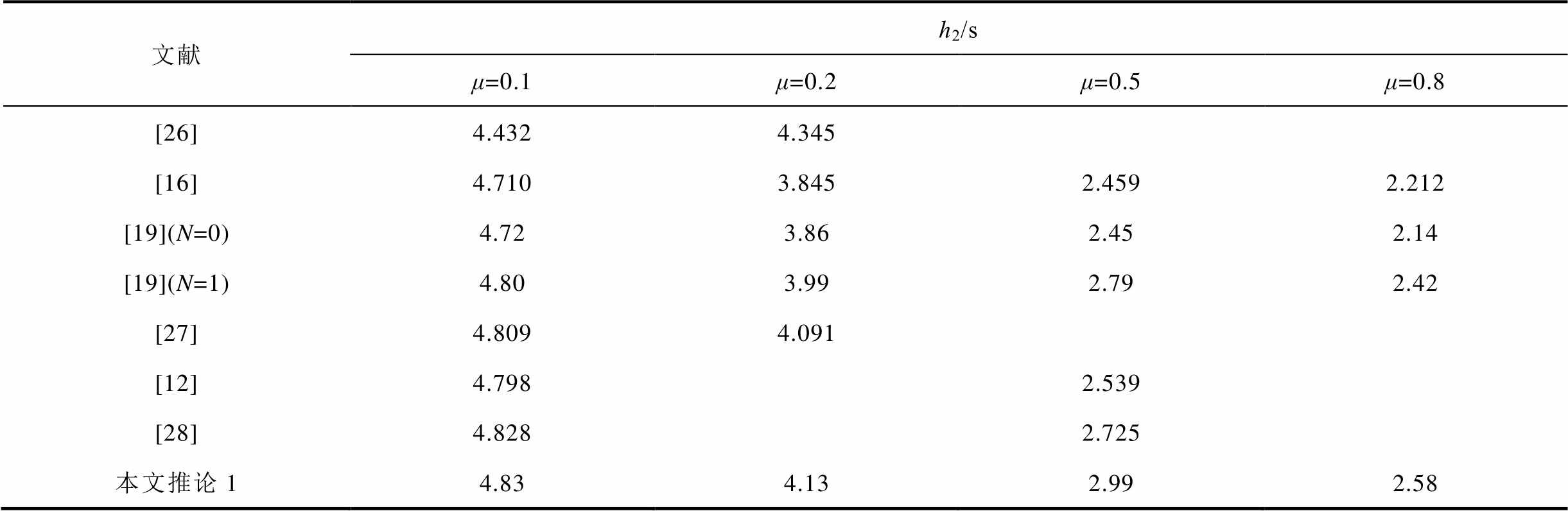
文献h2/s μ=0.1μ=0.2μ=0.5μ=0.8 [26]4.4324.345 [16]4.7103.8452.4592.212 [19](N=0)4.723.862.452.14 [19](N=1)4.803.992.792.42 [27]4.8094.091 [12]4.7982.539 [28]4.8282.725 本文推论14.834.132.992.58
从表2可以看出,当μ=0.5、h1取不同值时,推论1得到的时滞上界h2明显大于文献[11, 17-18, 23-25]的结果。从表3可以看出,当h1=0、μ取不同值时,推论1得到的时滞上界h2明显大于文献[12, 16, 19, 26-28]的结果。由此可见,本文方法得到的时滞上界更大,降低了现有结论的保守性。
从计算复杂性方面考虑,本文推论1决策变量个数为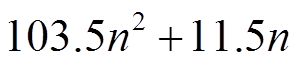 ,而文献[24]定理1、文献[28]定理4决策变量个数分别为
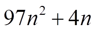 和
和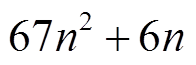 。由此可见,为了获得更大的时滞上界,本文的方法在一定程度上增加了计算复杂度。
考虑LFC系统,取实际系统的参数为Tch=0.3 s、Tg=0.1 s、 =0.05、D=1.0、β=21、M=10,表4给出了系统式(6)在时滞类型改变(μ=0、μ=0.5)、PI控制器参数(KP、KI)变化及不同扰动(σ、o)条件下,基于定理1得到的时滞上界对比数据,其中矩阵U=V=0.1I。由表4可以看出,固定时滞(μ=0)的上界要大于时变时滞(μ=0.5)的上界,即系统式(6)在固定时滞情况下具有更大的稳定裕度,且时滞上界随着σ、o的增大而减小,这说明负荷扰动对电力系统稳定性的影响是明显的。
表5和图2反映了PI控制器参数(KP、KI)与系统时滞上界的关系。当KP固定时,时滞上界h2随着KI增大而减小,且KP越小,这种趋势越明显。时滞上界h2与KP之间的关系更为复杂。当KI固定时,h2随着KP的增加先增大后减小。由此可见,PI控制器参数对时滞上界的影响非常明显。图2可以在不同的时滞上界时,为控制器参数KP、KI设计提供参考。
表4 不同条件下允许的时滞上界h2
Tab.4 Admissible upper bound h2 under different conditions
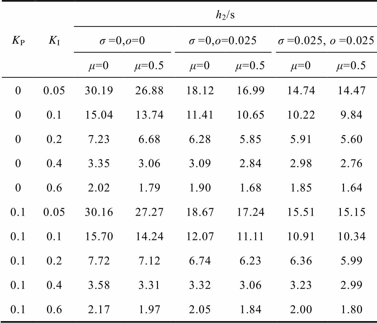
KPKIh2/s σ=0,ο=0σ=0,ο=0.025σ=0.025, ο=0.025 μ=0μ=0.5μ=0μ=0.5μ=0μ=0.5 00.0530.1926.8818.1216.9914.7414.47 00.115.0413.7411.4110.6510.229.84 00.27.236.686.285.855.915.60 00.43.353.063.092.842.982.76 00.62.021.791.901.681.851.64 0.10.0530.1627.2718.6717.2415.5115.15 0.10.115.7014.2412.0711.1110.9110.34 0.10.27.727.126.746.236.365.99 0.10.43.583.313.323.063.232.99 0.10.62.171.972.051.842.001.80
表5 KP、KI取不同值时允许的时滞上界h2
Tab.5 Admissible upper bound h2 under different KP and KI
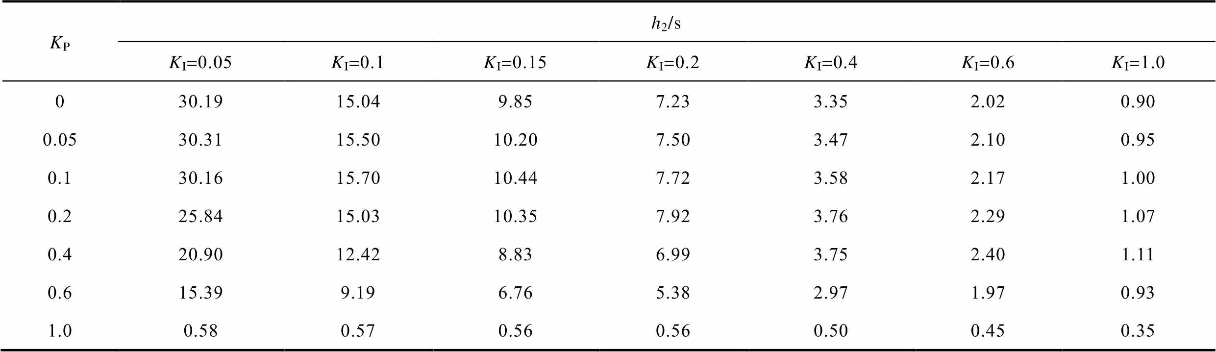
KPh2/s KI=0.05KI=0.1KI=0.15KI=0.2KI=0.4KI=0.6KI=1.0 030.1915.049.857.233.352.020.90 0.0530.3115.5010.207.503.472.100.95 0.130.1615.7010.447.723.582.171.00 0.225.8415.0310.357.923.762.291.07 0.420.9012.428.836.993.752.401.11 0.615.399.196.765.382.971.970.93 1.00.580.570.560.560.500.450.35
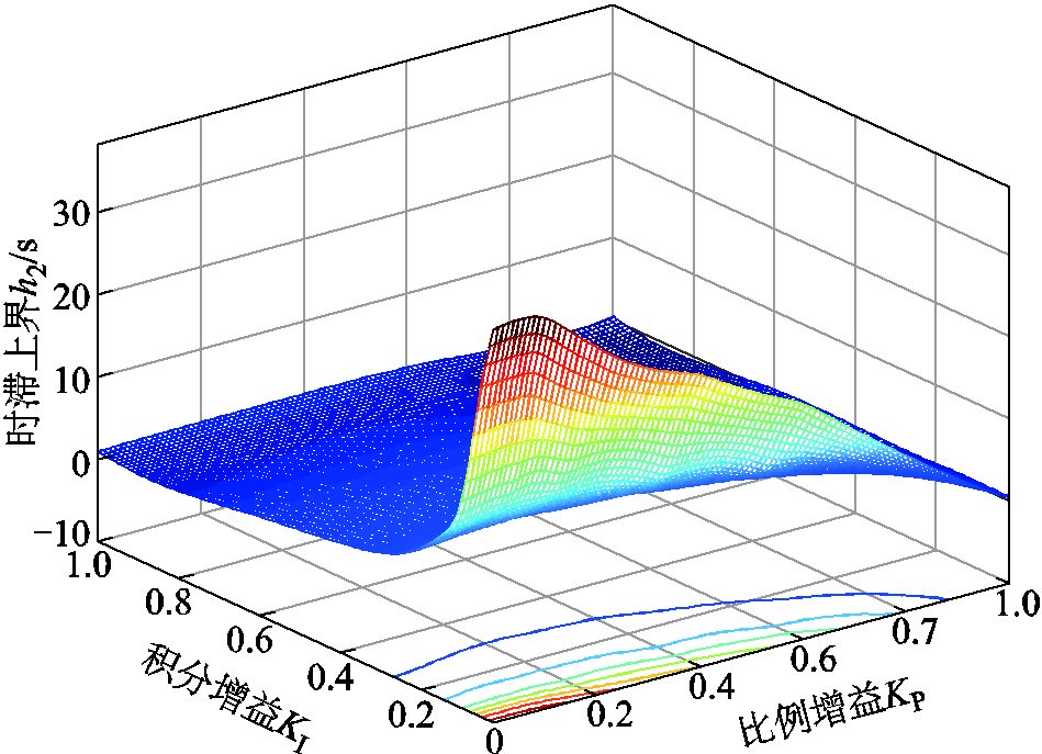
图2 控制器参数KP、KI与时滞上界h2的关系
Fig.2 Relationship among KP,KI and h2
表6、表7给出了本文定理1与现有文献[5,9,18, 29-30]得到的时滞上界对比数据。可以看出,由本文方法得到时滞上界大于其他方法,其中文献[5]采用Bessel-Legendre积分不等式,文献[9]运用基于Wirtinger积分不等式,文献[18]使用基于辅助函数的积分不等式,文献[29]运用Jensen不等式和反凸组合技术,文献[30]运用基于Wirtinger双重积分不等式。需要说明的是,表6、表7所列的时滞上界数据均为基于不同的方法得到估计值,并非系统时滞上界的真实值。越有效的方法得到的时滞上界越接近真实值,这也表明本文提出的新积分不等式在精确估计L-K泛函导数和提高稳定裕度方面具有优势。
表6 无负荷扰动系统KP、KI取不同值时,时滞上界h2结果对比
Tab.6 Comparative results of h2 with different KP, KI of no load disturbance system
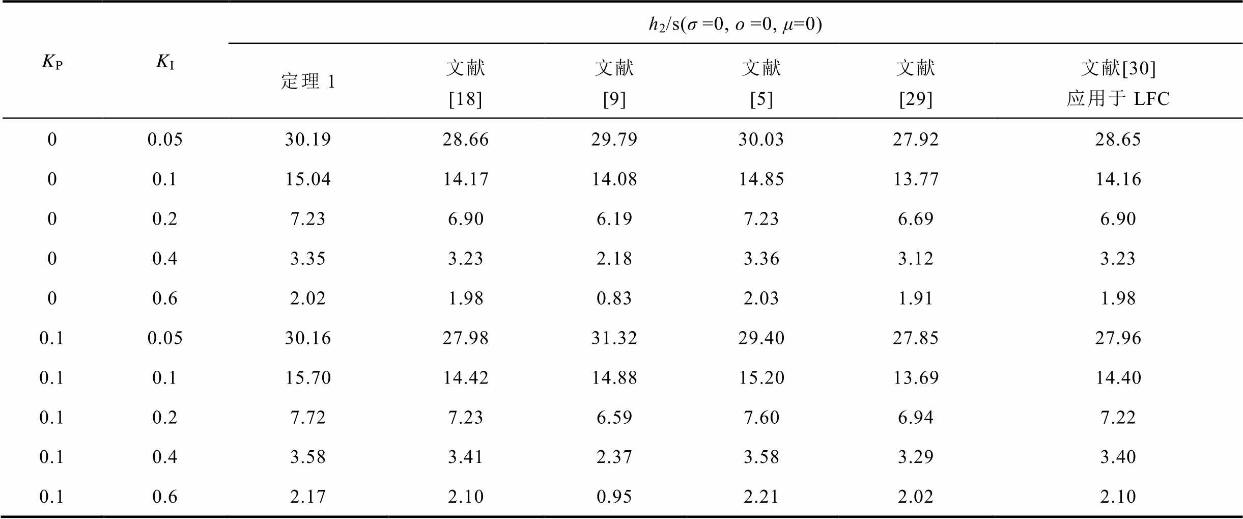
KPKIh2/s(σ=0, ο=0, μ=0)定理1文献 [18]文献 [9]文献 [5]文献 [29]文献[30]应用于LFC 00.0530.1928.6629.7930.0327.9228.65 00.115.0414.1714.0814.8513.7714.16 00.27.236.906.197.236.696.90 00.43.353.232.183.363.123.23 00.62.021.980.832.031.911.98 0.10.0530.1627.9831.3229.4027.8527.96 0.10.115.7014.4214.8815.2013.6914.40 0.10.27.727.236.597.606.947.22 0.10.43.583.412.373.583.293.40 0.10.62.172.100.952.212.022.10
表7 负荷扰动系统KP、KI取不同值时,时滞上界h2结果对比
Tab.7 Comparative results of h2 with different KP, KI of load disturbance system
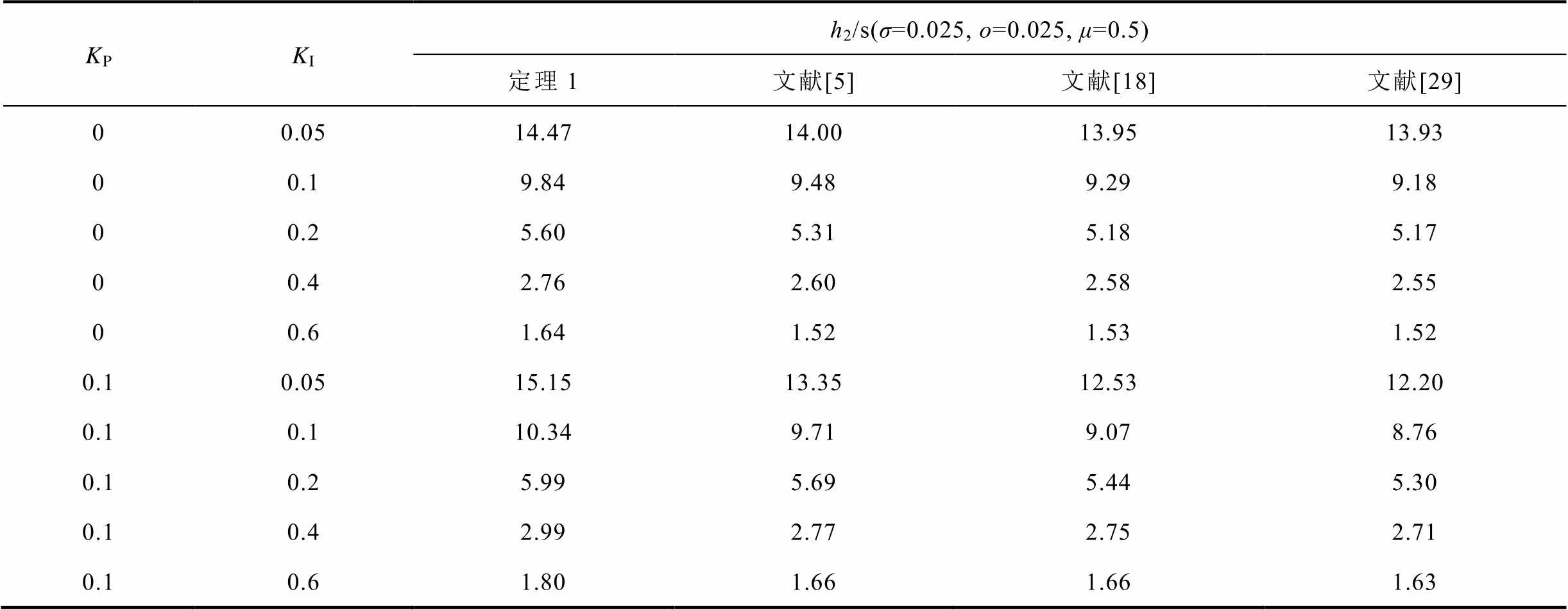
KPKIh2/s(σ=0.025, ο=0.025, μ=0.5)定理1文献[5]文献[18]文献[29] 00.0514.4714.0013.9513.93 00.19.849.489.299.18 00.25.605.315.185.17 00.42.762.602.582.55 00.61.641.521.531.52 0.10.0515.1513.3512.5312.20 0.10.110.349.719.078.76 0.10.25.995.695.445.30 0.10.42.992.772.752.71 0.10.61.801.661.661.63
表8给出了当,即不考虑负荷扰动情况下,取KP=0.1、KI=0.2时,由本文推论1、文献[14, 31]得到的无负荷扰动单区域LFC系统时滞上界数据。通过与文献[14, 31]的比较可以看出,推论1有效地提高了时滞上界,在一定程度上降低了稳定性判据的保守性。需要注意的是,本文新提出的方法也适用于时滞下界h1不限于零的情况。
表8 KP=0.1、KI=0.2,h1取不同值时,时滞上界h2结果对比
Tab.8 Comparative results of h2 with various h1 and KP=0.1, KI=0.2
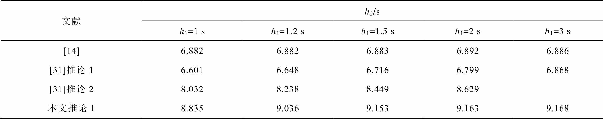
文献h2/s h1=1 sh1=1.2 sh1=1.5 sh1=2 sh1=3 s [14]6.8826.8826.8836.8926.886 [31]推论16.6016.6486.7166.7996.868 [31]推论28.0328.2388.4498.629 本文推论18.8359.0369.1539.1639.168
为了验证本文结果的准确性,针对单区域LFC系统模型,采用Matlab/Simulink进行仿真,分两种情况讨论。
1)时滞为恒定情况。选取负荷扰动参数U=0、 V=0.1I,标量σ=0、o=0.025。当KP=0.1、KI=0.4时,由表4可知系统的时滞上界h2=3.32 s。图3给出了该工况下频率偏差Δf的变化情况。可以看出,当时滞取上界3.32 s时,频率偏差收敛到零,系统渐近稳定;当时滞(3.60 s)超过上界值时,频率偏差出现振荡,无法收敛到零,系统不稳定。
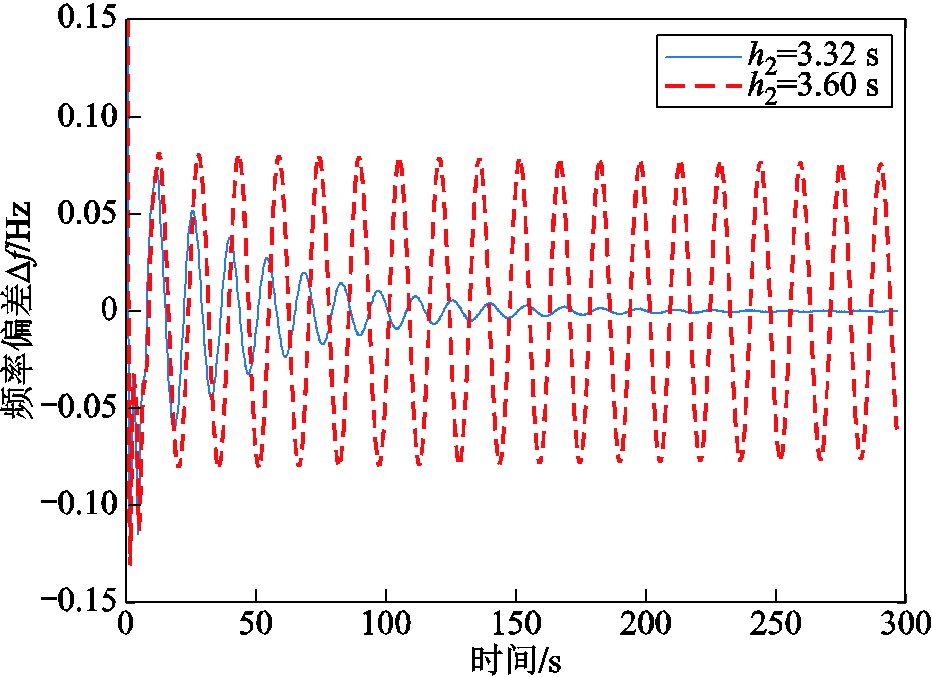
图3 固定时滞情况下频率响应曲线
Fig.3 Frequency response trajectory with constant delay
2)时滞为时变情况。选取负荷扰动参数U=V=0.1I,σ=o=0.025,当KP=0.1、KI=0.6时,由表4可知系统的时滞上界h2=1.80 s。图4给出了时滞随时间变化的系统式(6)的频率响应。可以看出,当时滞取上界1.80 s时,频率偏差收敛到零,系统渐近稳定;当时滞(2.20 s)超过上界值时,频率偏差出现振荡,无法收敛到零,系统不稳定。
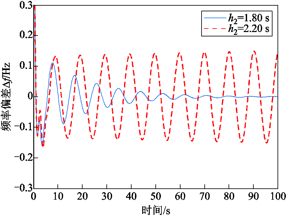
图4 时变时滞情况下频率响应曲线
Fig.4 Frequency response trajectory with time-varying delay
除了时滞对系统性能产生影响外,控制器参数也是影响系统性能的重要因素。为了验证PI控制器的比例增益KP、积分增益KI对频率偏差调节的影响,考虑固定时滞(μ=0)和无负荷扰动时(σ=0、o=0),在系统稳定的前提下,改变KP和KI,系统频率偏差动态响应如图5和图6所示。其中,图5给出了KP取相同值、KI取不同值时,系统频率偏差响应曲线。可以看出,KI越大,系统超调量越小,稳态误差消除得越快。
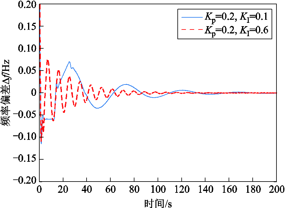
图5 相同KP、不同KI时频率响应曲线
Fig.5 Frequency response trajectory with the same KPand different KI
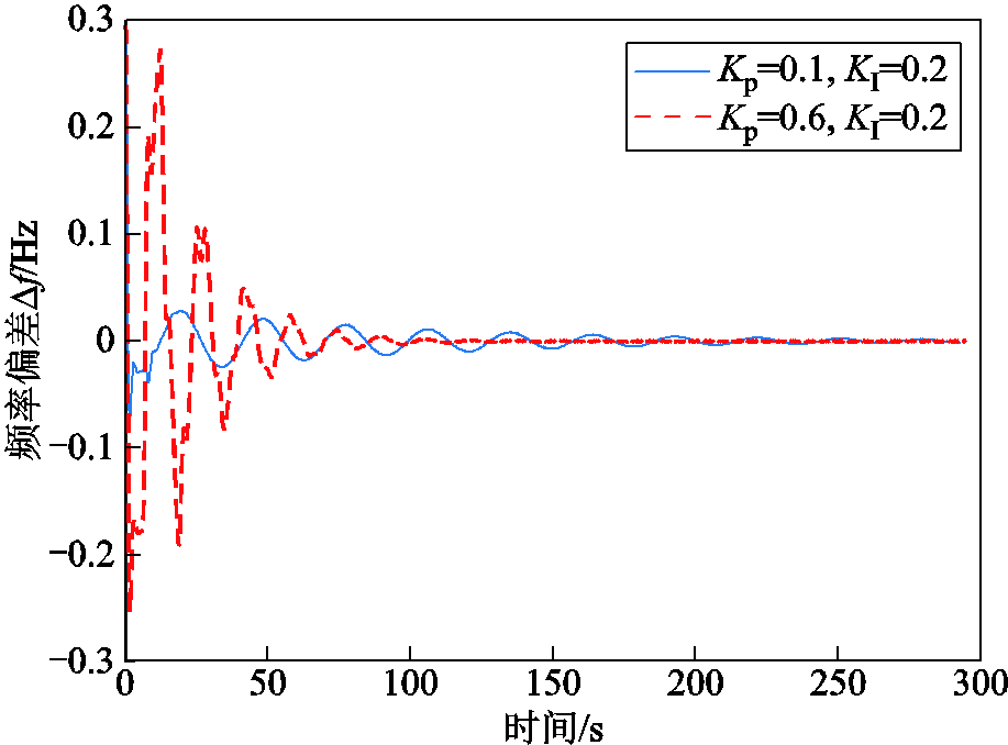
图6 相同KI、不同KP时频率响应曲线
Fig.6 Frequency response trajectory with the same KI and different KP
图6给出了KI取相同值、KP取不同值时,系统频率偏差响应曲线。可以看出,KP越大,系统响应速度越快,趋于稳定的时间越短,但在初始阶段,出现了较大的超调量。
本文研究了时滞LFC系统的稳定性问题。通过构造增广向量和具有多重积分项的L-K泛函,增强了不同变量间的耦合关系,为得到保守性小的稳定性判据奠定了基础。处理泛函导数时,在传统自由矩阵积分不等式和反凸组合技术基础上进行拓展延伸,提出了新的DDMB和FMB积分不等式、EDDMB反凸组合不等式,通过引入时滞相关自由矩阵,充分利用更多的时滞信息,从而使泛函导数估计更加精确,进而得到了保守性更小的结论。仿真结果表明了该方法的有效性和优越性。需要注意的是,该方法在一定程度上增加了计算量。如何在L-K泛函中减少冗余矩阵,从而在保证稳定裕度不变的前提下,减小计算量,并考虑LFC系统中非线性和随机出现的不完全信息等其他因素,是需要在今后工作中进一步研究的问题。此外,本文仅讨论了LFC系统各区域时滞均相同的情况,在实际系统中,还存在多时滞、混合时滞及随机时滞等更为复杂的情况,这也是需要进一步深入研究探讨的问题。
附 录
定理1证明如下。
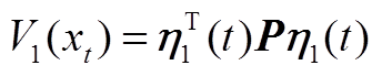
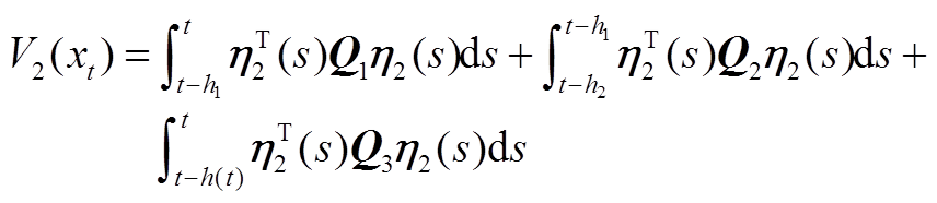
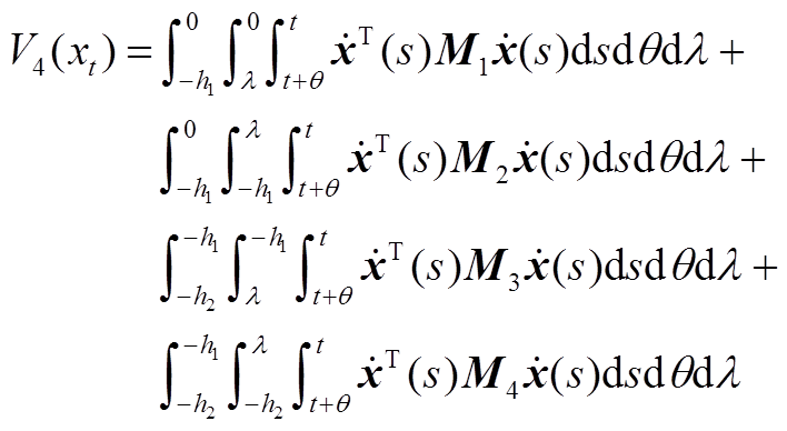
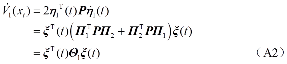
针对系统式(6)构造L-K泛函为
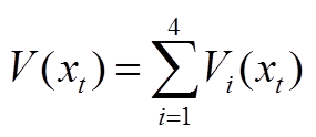 (A1)
(A1)
其中

显然, 成立。
成立。
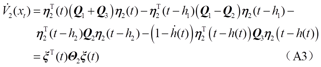
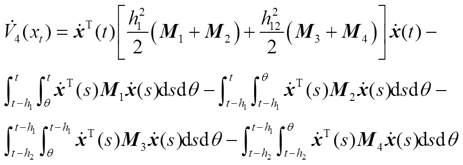
沿着系统式(6)解轨线对 求导可得
求导可得
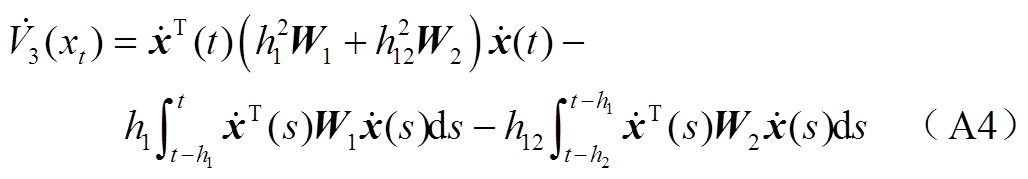
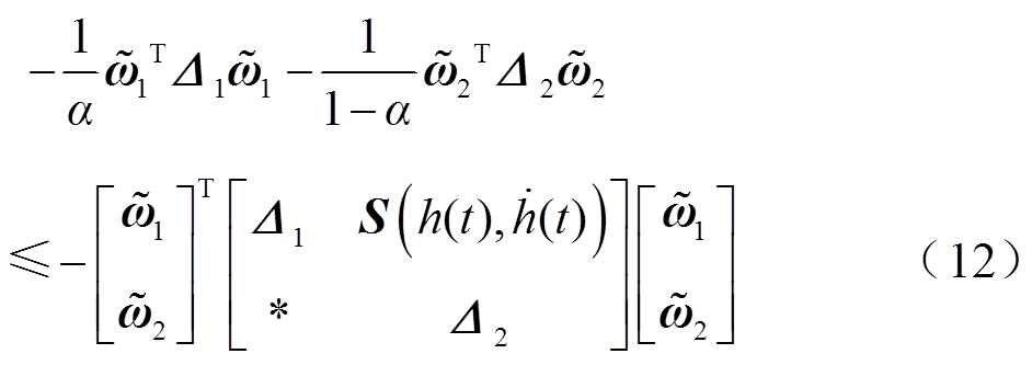
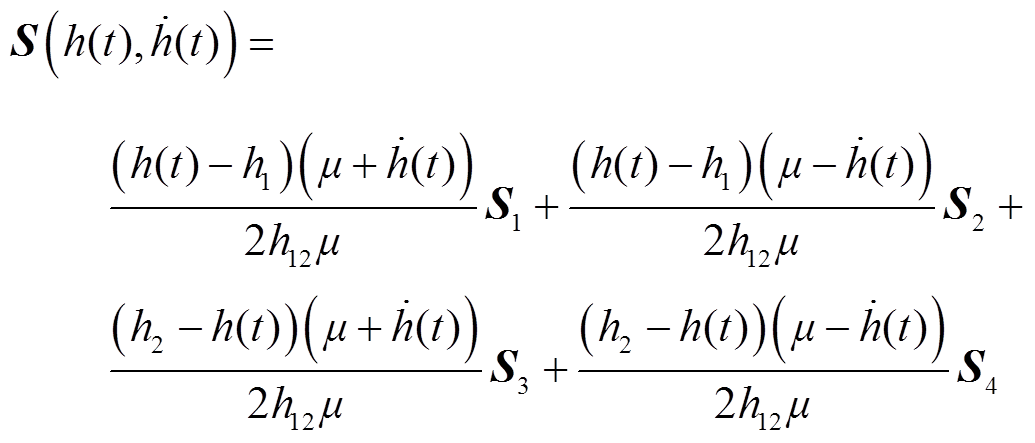
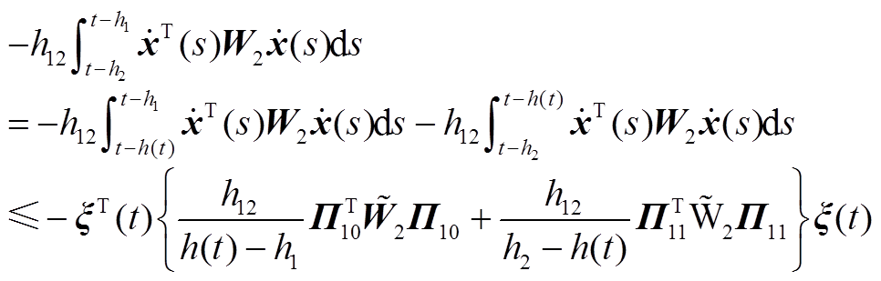
考虑式(A4)中第一个积分项,根据命题1可得
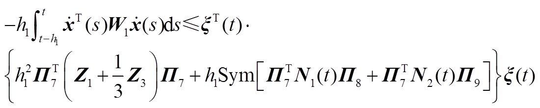 (A5)
(A5)
考虑式(A4)中第二个积分项,根据引理1和命题2可得
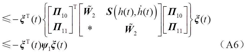
由式(A4)~式(A6)可得
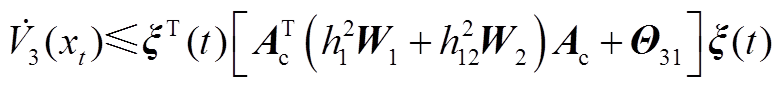 (A7)
(A7)
对 求导得到
求导得到
 (A8)
(A8)
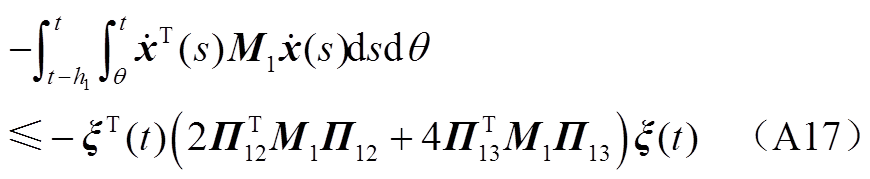
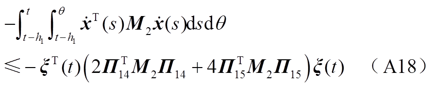
将式(A8)中后两项二重积分的积分区间进行分割,得到
 (A9)
(A9)
 (A10)
(A10)
 (A11)
(A11)
 (A12)
(A12)
 (A13)
(A13)
 (A14)
(A14)
 (A15)
(A15)
 (A16)
(A16)
运用引理2对 中的二重积分进行估计可得
 (A19)
(A19)
 (A20)
(A20)
 (A21)
(A21)
 (A22)
(A22)
同时,运用引理3对 、
、 进行估计可得
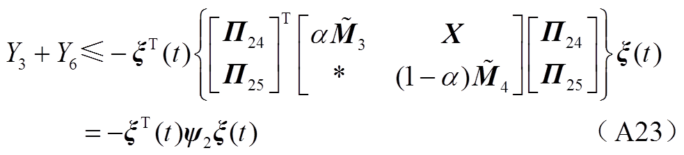
将式(A9)~式(A23)代入式(A8)可得
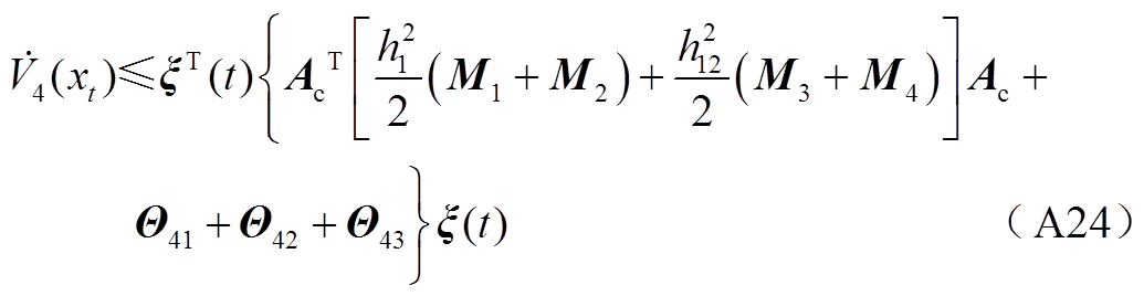
结合式(A2)、式(A3)、式(A7)和式(A24)可得到
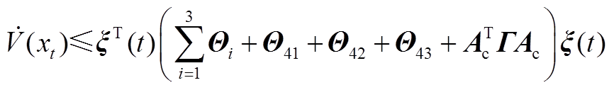 (A25)
(A25)
因,故当 时,系统式(6)渐近稳定,即
 (A26)
(A26)
利用Schur补引理,式(A26)等价于式(17),证明完毕。
需要注意的是,众所周知,构造合适的L-K泛函是降低稳定性判据保守性的关键。本文 的增广向量中引入了单重积分项
 、
、 和二重积分项
 、
、 ,从而在不同的变量间建立了更多的耦合关系。相比于文献[18]中的单重积分项
 ,本文将
,本文将 增广为
增广为 ,加强了泛函与系统的信息联系。此外,
 和分别为双重和三重积分泛函,从而更好地利用了时滞信息。上述这些L-K泛函构造方法,对于降低系统的保守性将起到重要作用。
此外,本文利用DDMB和FMB积分不等式估计 中的单重积分项
 ,引入了时滞相关矩阵,有效利用了时滞
 及其导数
及其导数 信息。在处理
 时,将积分区间分割成[t-h2, t-h(t)]和[t-h(t), t-h1]两个子区间,然后应用基于辅助函数的单重积分不等式和本文提出的EDDMB反凸组合不等式配合处理,有效地提高了估计精度。
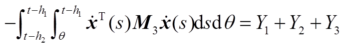
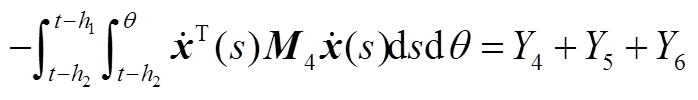
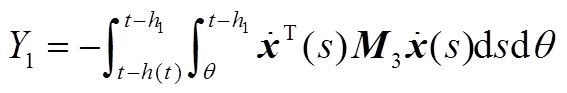
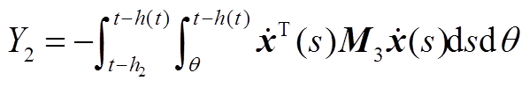
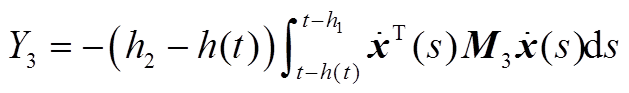
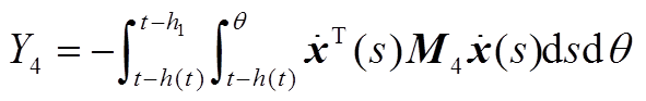
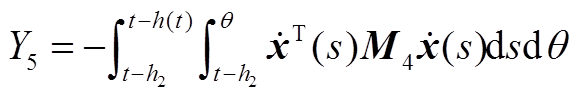
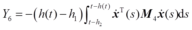
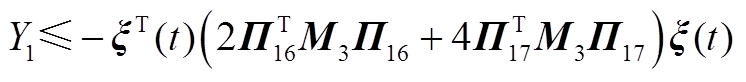
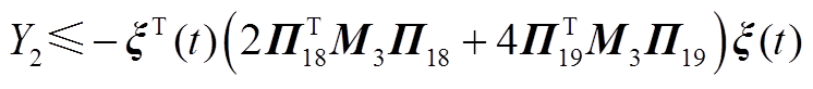
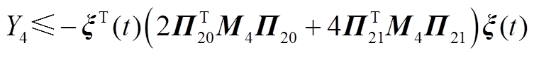
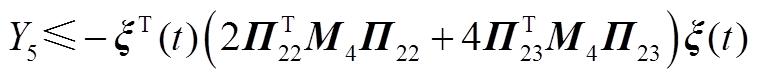
最后,现有的一些文献在构造L-K泛函时引入三重积分项,但在推导过程中对其导数进行直接放缩,没有充分利用时滞信息,从而导致了结果的保守性。本文在对 进行放缩处理时,将三重积分的导数
 、
、 分别分割成Y1、Y2、Y3和Y4、Y5、Y6,从而充分地利用了时滞信息。此外,利用基于辅助函数的二重积分不等式估计了Y1、Y2、Y4、Y5,利用松弛积分不等式估计了Y3+Y6,进一步提高估计精度,降低了结果的保守性。
参考文献
[1] 陈宗遥, 卜旭辉, 郭金丽. 基于神经网络的数据驱动互联电力系统负荷频率控制[J]. 电工技术学报, 2022, 37(21): 5451-5461. Chen Zongyao, Bu Xuhui, Guo Jinli. Neural network based data-driven load frequency control for interconnected power systems[J]. Transactions of China Electrotechnical Society, 2022, 37(21): 5451-5461.
[2] 常烨骙, 李卫东, 巴宇, 等. 基于运行安全的频率控制性能评价新方法[J]. 电工技术学报, 2019, 34(6): 1218-1229. Chang Yekui, Li Weidong, Ba Yu, et al. A new method for frequency control performance assessment on operation security[J]. Transactions of China Electrotechnical Society, 2019, 34(6): 1218-1229.
[3] 梁煜东, 陈峦, 张国洲, 等. 基于深度强化学习的多能互补发电系统负荷频率控制策略[J]. 电工技术学报, 2022, 37(7): 1768-1779. Liang Yudong, Chen Luan, Zhang Guozhou, et al. Load frequency control strategy of hybrid power generation system: a deep reinforcement learning-based approach[J]. Transactions of China Electrotechnical Society, 2022, 37(7): 1768-1779.
[4] 吕永青, 窦晓波, 杨冬梅, 等. 含荷电状态修正和通信延迟的储能电站负荷频率鲁棒控制[J]. 电力系统自动化, 2021, 45(10): 59-67. Lü Yongqing, Dou Xiaobo, Yang Dongmei, et al. Load-frequency robust control for energy storage power station considering correction of state of charge and communication delay[J]. Automation of Electric Power Systems, 2021, 45(10): 59-67.
[5] Yang Feisheng, He Jing, Pan Quan. Further improvement on delay-dependent load frequency control of power systems via truncated B-L inequality[J]. IEEE Transactions on Power Systems, 2018, 33(5): 5062-5071.
[6] Hua Changchun, Wang Yibo, Wu Shuangshuang. Stability analysis of micro-grid frequency control system with two additive time-varying delay[J]. Journal of the Franklin Institute, 2020, 357(8): 4949-4963.
[7] 马燕峰, 霍亚欣, 李鑫, 等. 考虑时滞影响的双馈风电场广域附加阻尼控制器设计[J]. 电工技术学报, 2020, 35(1): 158-166. Ma Yanfeng, Huo Yaxin, Li Xin, et al. Design of wide area additional damping controller for doubly fed wind farms considering time delays[J]. Transactions of China Electrotechnical Society, 2020, 35(1): 158-166.
[8] 钱伟, 王晨晨, 费树岷. 区间变时滞广域电力系统稳定性分析与控制器设计[J]. 电工技术学报, 2019, 34(17): 3640-3650. Qian Wei, Wang Chenchen, Fei Shumin. Stability analysis and controller design of wide-area power system with interval time-varying delay[J]. Transactions of China Electrotechnical Society, 2019, 34(17): 3640-3650.
[9] Luo Haocheng, Hiskens I A, Hu Zechun. Stability analysis of load frequency control systems with sampling and transmission delay[J]. IEEE Transactions on Power Systems, 2020, 35(5): 3603-3615.
[10] Shen Hao, Chen Mengshen, Wu Zhengguang, et al. Reliable event-triggered asynchronous extended passive control for semi-markov jump fuzzy systems and its application[J]. IEEE Transactions on Fuzzy Systems, 2020, 28(8): 1708-1722.
[11] Qian Wei, Yuan Manman, Wang Lei, et al. Stabilization of systems with interval time-varying delay based on delay decomposing approach[J]. ISA Transactions, 2017, 70: 1-6.
[12] Kwon O M, Lee S H, Park M J, et al. Augmented zero equality approach to stability for linear systems with time-varying delay[J]. Applied Mathematics and Computation, 2020, 381: 125329.
[13] Qian Wei, Xing Weiwei, Fei Shumin. H(∞) state estimation for neural networks with general activation function and mixed time-varying delays[J]. IEEE Transactions on Neural Networks and Learning Systems, 2021, 32(9): 3909-3918.
[14] Xu Haotian, Zhang Chuanke, Jiang Lin, et al. Stability analysis of linear systems with two additive time-varying delays via delay-product-type Lyapunov functional[J]. Applied Mathematical Modelling, 2017, 45: 955-964.
[15] Zhang Zhiming, He Yong, Wu Min, et al. Exponential synchronization of neural networks with time-varying delays via dynamic intermittent output feedback control[J]. IEEE Transactions on Systems, Man, and Cybernetics: Systems, 2019, 49(3): 612-622.
[16] Zeng Hongbing, He Yong, Wu Min, et al. Free-matrix-based integral inequality for stability analysis of systems with time-varying delay[J]. IEEE Transactions on Automatic Control, 2015, 60(10): 2768-2772.
[17] Qian Wei, Gao Yanshan, Chen Yonggang, et al. The stability analysis of time-varying delayed systems based on new augmented vector method[J]. Journal of the Franklin Institute, 2019, 356(3): 1268-1286.
[18] Yang Feisheng, He Jing, Wang Jing, et al. Auxiliary-function-based double integral inequality approach to stability analysis of load frequency control systems with interval time-varying delay[J]. IET Control Theory & Applications, 2018, 12(5): 601-612.
[19] Seuret A, Gouaisbaut F. Stability of linear systems with time-varying delays using Bessel-Legendre inequalities[J]. IEEE Transactions on Automatic Control, 2018, 63(1): 225-232.
[20] Zhang Ruimei, Zeng Deqiang, Park J H, et al. New approaches to stability analysis for time-varying delay systems[J]. Journal of the Franklin Institute, 2019, 356(7): 4174-4189.
[21] Yang Feisheng, He Jing, Wang Dianhui. New stability criteria of delayed load frequency control systems via infinite-series-based inequality[J]. IEEE Transactions on Industrial Informatics, 2018, 14(1): 231-240.
[22] Jin Li, Zhang Chuanke, He Yong, et al. Delay-dependent stability analysis of multi-area load frequency control with enhanced accuracy and computation efficiency[J]. IEEE Transactions on Power Systems, 2019, 34(5): 3687-3696.
[23] van Hien L, Trinh H. Refined Jensen-based inequality approach to stability analysis of time-delay systems[J]. IET Control Theory & Applications, 2015, 9(14): 2188-2194.
[24] Liu Yajuan, Park J H, Guo Baozhu. Results on stability of linear systems with time varying delay[J]. IET Control Theory & Applications, 2017, 11(1): 129-134.
[25] Kwon O M, Park M J, Park J H, et al. Enhancement on stability criteria for linear systems with interval time-varying delays[J]. International Journal of Control, Automation and Systems, 2016, 14(1): 12-20.
[26] Abolpour R, Dehghani M, Talebi H A. Stability analysis of systems with time-varying delays using overlapped switching Lyapunov Krasovskii functional[J]. Journal of the Franklin Institute, 2020, 357(15): 10844-10860.
[27] Zhang Chuanke, He Yong, Jiang Lin, et al. Notes on stability of time-delay systems: bounding inequalities and augmented Lyapunov-Krasovskii functionals[J]. IEEE Transactions on Automatic Control, 2017, 62(10): 5331-5336.
[28] Gyurkovics É, Takács T. Comparison of some bounding inequalities applied in stability analysis of time-delay systems[J]. Systems & Control Letters, 2019, 123: 40-46.
[29] Ramakrishnan K, Ray G. Stability criteria for nonlinearly perturbed load frequency systems with time-delay[J]. IEEE Journal on Emerging and Selected Topics in Circuits and Systems, 2015, 5(3): 383-392.
[30] Park M J, Kwon O M, Park J H, et al. Stability of time-delay systems via Wirtinger-based double integral inequality[J]. Automatica, 2015, 55: 204-208.
[31] Qian Wei, Xing Weiwei, Wang Lei, et al. New optimal analysis method to stability and H(∞) performance of varying delayed systems[J]. ISA Transactions, 2019, 93: 137-144.
Abstract In wide-area interconnected power systems, load frequency control (LFC) has a pivotal role in addressing the issue of upholding the variations in system frequency and power exchange between different control areas at desired scheduled values. With the development of smart grid technologies and the emergence of numerous private networks, open communication networks are widely used, which inevitably leads to communication delay. The communication delay is an important factor affecting the stability and performance of LFC system. At present, Lyapunov-Krasovskii (L-K) functional method is one of the main methods to study the stability of LFC system. To this issue, how to construct appropriate L-K functional and estimate the functional derivatives accurately to reduce the conservatism of conclusions is the core problem, and the sustained efforts have been made, but it is far from enough in how to coordinate functional construction with estimating techniques efficiently. In this paper, the stability problem of LFC system with delay influence and load disturbance is further studied, by proposing some new methods, the less conservative stability criteria are obtained, and the influence of controller parameters on the delay margin is analyzed.
Firstly, by considering time delay and load disturbance, the LFC system model is established. Secondly, a new L-K functional with augmented vector and multiple integral terms is constructed. The single integral terms and the double integral terms are introduced, which builds more relations among different vectors. Moreover, state vector and its derivative are augmented to deepen the relationships between L-K functional and the system. Besides, integral functionals with double and triple forms are also created to get a better exploitation of delay information, all of which conduce to the stability criteria with less conservatism.
Then, in order to cooperate with the constructed functional effectively, two inequalities named delay-dependent-matrix-based and free-matrix-based integral inequality (DDMB and FMB integral inequality) and extended delay-dependent-matrix-based reciprocally convex inequality (EDDMB reciprocally convex inequality) are proposed to estimate the functional derivatives more accurately. Compared with the existing estimation approaches with constant matrices, DDMB and FMB integral inequality employs delay-dependent matrices and utilizes more information of time delay and its derivative, which provides more freedom in reducing the conservatism of the main results.Compared with the existing DDMB reciprocally convex inequality, EDDMB reciprocally convex inequality is more general because the value of delay lower bound is relaxed, which expands its scope of application. In addition, auxiliary-function-based integral inequalities (AFBII) together with relaxed integral inequality are also used, which helps to get less conservative stability conditions.
The simulation of typical second-order delay system and single-region delay LFC system are given, and the influence of load disturbance and controller parameters on the upper bound of single-region delayed LFC system under different conditions is analyzed. The following conclusions can be drawn from the simulation analysis: (1) Compared with the research results of some existed literatures, the upper bound of time delay obtained by the proposed method is significantly larger, which indicates that the proposed method can effectively improve the stability margin of time delay and reduce the conservatism of the conclusion. (2) The influence of load disturbance and controller parameters on the upper bound of system delay is obvious, the larger the load disturbance is, the smaller the upper bound of system delay is. When the PI control is applied, the upper bound of time delay decreases with the increase of integral gain, and this trend is more obvious when the proportional gain is smaller. The relation between the upper bound of time delay and the proportional gain is more complicated, the upper bound of time delay increases first and then decreases with the increase of the proportional gain.
keywords:Power system stability, load frequency control, time-varying delay, Lyapunov-Krasovskii functional, delay-dependent-matrix-based
DOI:10.19595/j.cnki.1000-6753.tces.220811
中图分类号:TM712
国家自然科学基金项目(61973105)、河南省创新型科技团队项目(CXTD2016054)和河南省科技攻关项目(232102240096)资助。
收稿日期 2022-05-14
改稿日期 2022-09-26
郭建锋 男,1980年生,博士研究生,研究方向为电力系统分析与控制。E-mail:gjf@hpu.edu.cn
钱 伟 男,1978年生,博士,教授,博士生导师,研究方向为鲁棒控制、智能控制。E-mail:qwei@hpu.edu.cn(通信作者)
(编辑 李冰)