 (1)
(1)
Abstract For permanent magnet synchronous machines (PMSMs), the speed operation range can hardly be extended due to the increasing back electromotive force and the limited DC link voltage. The flux-weakening method is employed to extend the speed operation range and maximize the torque capability. Based on the conventional current vector control system, the flux-weakening control methods can be achieved in both feedforward and feedback manners. Compared to the feedforward type flux-weakening control method, the feedback type flux-weakening control method is simple and more robust in performance against parameter mismatches. For feedback type flux-weakening control, there are two main control methods, i.e., dq-axis current-based feedback flux-weakening control (DQFFC) and current amplitude and angle-based feedback flux-weakening control (CAAFFC), which are considered to be equivalent to each other. In this paper, the system stabilities of the two methods are comparatively studied by considering maximum torque per voltage (MTPV) control and over-modulation, and the control parameter design for DQFFC and CAAFFC is discussed.
In this paper, based on the current vector control system, the basic principles of the two feedback-type flux-weakening methods are introduced, and the operation modes and regions of the two flux-weakening control methods are defined and illustrated. Secondly, the voltage feedback control loops of DQFFC and CAAFFC are generalized and linearized, and the corresponding transfer functions are derived. Thirdly, based on the derived transfer function, the stability characteristics of the two flux-weakening control methods are analyzed by applying the Routh stability criterion. In the analysis, the stabilities of the two flux-weakening control methods at different operation regions are compared and illustrated from the perspective of d- and q-axis current regulations. Based on the stability analysis, control parameters for DQFFC and CAAFFC are designed, respectively. The analysis indicates that DQFFC and CAAFFC show different regional stability characteristics. Moreover, it is found that the instabilities can be caused by not only the control parameters of flux-weakening control methods but also the flux-weakening control methods inherently.
From both the theoretical analysis and experiment results, it can be confirmed that the instability characteristics can be different between these two flux-weakening control methods in two different operation regions. Firstly, when the current approaches the MTPV curve, the DQFFC method has a weak voltage regulation capability since only the d-axis current can be regulated. The current can be prevented from moving inside the voltage limit circle, causing oscillation in over-modulation. On the other hand, the CAAFFC method mainly regulates the q-axis current in this region, allowing the current to move within the voltage limit circle. Thus, the oscillation can be alleviated. Secondly, when the machine operates under a light load condition, the CAAFFC method mainly regulates the q-axis current, and the current cannot move inside the voltage limit circle, which causes an unstable transition between motoring and generating modes. On the other hand, DQFFC with d-axis current regulation has no issues since the current can move within the voltage limit circle. Thus, a smooth and stable transition can be achieved.
keywords:Flux weakening, instability, maximum torque per voltage (MTPV), oscillation, permanent magnet synchronous machine (PMSM), stability, voltage feedback controller
Permanent magnet synchronous machines (PMSMs) are widely used in applications, such as electric vehicles, aerospace, and household applications, due to high efficiency and high power and torque densities[1-4]. However, the speed operation range can be hardly extended due to the increasing back electromotive force and the limited DC link voltage. To extend the speed operation range and maximize the torque capability, the flux-weakening method is normally employed without the requirement to Boost the DC-link voltage[5-40].
Based on the conventional current vector control system, the flux-weakening control requires modi- fying the current trajectory to satisfy the current and voltage constraints[7]. The flux-weakening methods can be mainly categorized as feedforward[7-11], feedback[14-27], and hybrid method[32-35]. However, although the feedforward method can obtain fast dynamics[11], they suffer from the variations of the machine parameters. The stable operation of the feedforward method normally requires enough voltage margin to tolerate the deviation of the parameters[12]. Therefore, the torque capability in the flux-weakening region can be hardly maximized. The method in Ref.[13] based on the feedforward method is further optimized by online adjusting the current reference with certain performance criteria. However, it requires many decision trees and the proper criteria require much tuning work. On the other hand, the feedback method is robust to parameter variations due to a closed-loop structure. The input of the feedback controller can be the voltage magnitude error[14-23], the voltage error before and after over modulation block[24-26], the error between the switching period and summation of active switching times for the inverter pulse width modulation (PWM)[27]. The latter two feedback methods are specifically designed for the over modulation flux-weakening operation, it cannot achieve the linear modulation operation. Since the operation region for the voltage magnitude feedback method depends on the given voltage magnitude reference, it can operate in either linear or over modulation region. Even in the linear modulation region, the voltage magnitude feedback method is recommended to leave a certain voltage margin for the current control[12, 14-15]. The less voltage margin could lead to conflict between the d- and q-axis current controllers, which could result in oscillation. Therefore, other methods such as the single current controller (SCC) method[28] and the voltage angle control method[29-30] are proposed to solve this conflict by using only one current controller. In the SCC method, the optimal q-axis voltage reference is given with a value that relies on machine parameters. The voltage angle control cannot guarantee the current dynamics and generally shows poorer current dynamics than the conventional dual-current control structure[17]. InRef.[31], the current dynamics for the voltage angle control are improved by adding a feedforward high pass filter processed d-axis current to the voltage angle. However, it requires proper criteria to achieve a smooth transition between the constant torque region and the flux-weakening region. InRef.[17], a voltage vector modifier (VVM) is proposed to improve the current dynamics in the over modulation region, by which even the six-step operation can be achieved and the dual-current control structure is still preserved. The hybrid methods in Ref.[32-35] contain both forward and feedback paths. The current feedforward components are normally achieved by 2-D look-up tables that can be obtained through finite element results or offline experimental results which can further improve the torque control accuracy. The feedback path gains the tolerance for the parameter variations, and therefore improves the system stability. The improved performance of the hybrid method is at the expense of flexibility and simplicity.
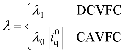
In this paper, the traditional voltage magnitude feedback method is be focused on, owing to its advantages of simple, robust, and standard control structure. However, due to the voltage and current constraints in the flux-weakening region, the system operates on the boundary between linearity and nonlinearity, especially in the over modulation region. The stability of the feedback control becomes an important issue which directly affects the reliability of the flux-weakening method. Conventionally, two variants of the voltage feedback controller, i.e. d-axis current based voltage feedback controller (DCVFC)[14-19] and current angle based voltage feedback controller (CAVFC)[20-23], are normally considered to be equivalent to achieve flux-weakening operation. However, the differences between DCVFC and CAVFC from the stability point of view are seldom discussed, especially when the maximum torque per voltage (MTPV) control is considered. By further considering the MTPV control, in this paper, two feedback-type flux-weakening methods, i.e. dq-axis currents based feedback flux-weakening control (DQFFC), current amplitude and angle based feedback flux-weakening control (CAAFFC), are introduced and comparatively studied in terms of the system stability on a non-salient PMSM. In addition, the feedback-type MTPV controllers in DQFFC and CAAFFC are analyzed and designed. Since the VVM in Ref.[17] is based on the DCVFC and a PM machine with finite constant power speed ratio (CPSR), it does not consider the machine with infinite CPSR, i.e. with MTPV control. Therefore, in this paper, the effectiveness of the VVM on the two different flux-weakening methods in the over modulation region is also compared. The analysis indicates that DQFFC and CAAFFC show different stability characteristics in different regions. The oscillation and instability could occur for the DQFFC and CAAFFC, respectively, under different regions.
This paper is organized as follows. Firstly, based on the current vector control system, two feedback- type flux-weakening methods are introduced. Secondly, the stability of the voltage loop in DQFFC and CAAFFC are comparatively studied, and the corre- sponding MTPV controllers are designed. Thirdly, the experimental validation is presented. Finally, the conclusions are drawn.
The mathematical model of non-salient PMSM in the dq-axis synchronous reference frame can be expressed as
(1)
where V, i are the stator voltage and current, respectively; the subscripts ‘d’ and ‘q’ indicate the relevant components in d- and q-axis; Rs is the stator resistance;Ls is the synchronous inductance; weis the electrical angular speed; ymis the permanent magnet flux linkage; TL is the load torque; J is the moment of inertia; np is the number of pole pairs.
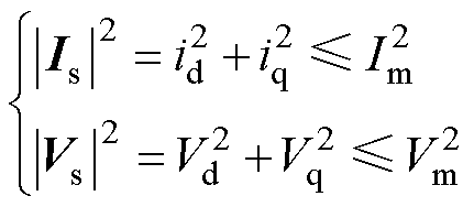
There are two supply constraints, i.e. current and voltage limits, which can be written as
 (2)
(2)
where Is and Vs are the current and voltage vectors,i.e.id+jiq and Vd+jVq in the dq-axis frame; Imis the current limit; Vmis the voltage limit which is restricted by the DC-link voltage Vdc and the over modulation methods[41].
Fig.1 shows the operation regions in the whole speed range with consideration of MTPV.

Fig.1 Operation regions
The whole operation region can be divided into three parts, i.e. regions Ⅰ, Ⅱ, and Ⅲ. In region I, the machine operates on the curve ‘OA’, aiming to achieve the maximum torque per ampere (MTPA). Region Ⅱ includes the curve ‘AB’ and the area within the closed curve ‘OABCO’. On the curve ‘AB’, the machine operates on the intersection point of the voltage and current limit circle, i.e.|Vs|=Vm and |Is|=Im. In the area ‘OABCO’, the machine operates on the voltage limit circle and inside the current limit circle, i.e. |Vs|=Vm and |Is|<Im. In region Ⅲ, the machine operates on the MTPV curve ‘BC’ inside the current limit circle, i.e. |Is|<Im and |Vs|=Vm.
Fig.2 shows the schematic of a current vector control system with flux-weakening control. The output of the speed proportion-integral (PI) controller is the current command  . Thedq-axis current commands, i.e.
  and
and  ,come from theflux- weakening block with the proper flux-weakening methods. The minimum phase error over modulation (MPEOM) is employed as the over modulation method[41]. A VVM[17] is adopted to improve the current dynamics in the over modulation region for the machine without MTPV control. In this paper, the VVM will also be used for the machine with MTPV control. The working principle of the VVM is shown in Fig.3. In Fig.3, the voltage command vector
  output from the current regulator is limited by the hexagon boundary and will be truncated to the voltage vector Vstmp, which is regarded as the temporal voltage vector. Then, the modified voltage vector
  is obtained by adding a rotated 90 ° temporal voltage error vector to the original voltage vector. Hence, the modified voltage vector is obtained as
 (3)
(3)
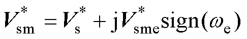
where =-Vstmpis the temporal voltage error vector. Therefore, as shown in Fig.3, the VVM converts the unrealizable voltage magnitude command to the voltage angle command
  while the dual-currentcontrol structure is still maintained, which therefore Boosts the current dynamics and enhances the system stability in over modulation region. It should be noted that the voltage modifier only takes effect when the system operates in the over modulation region and will not affect the system performance in the linear modulation region.
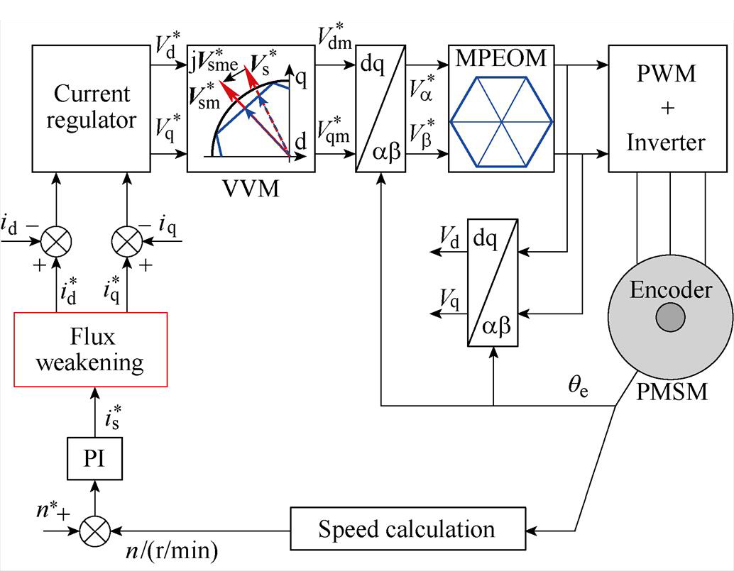
Fig.2 Schematic of current vector control system with flux weakening
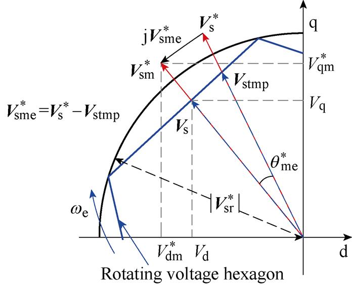
Fig.3 Voltage vector modifier (VVM)
Fig.4 shows the block diagrams of two feedback flux-weakening methods, i.e. DQFFC and CAAFFC. The MTPV control strategy in DQFFC and CAAFFC is achieved by forcing the MTPV penalty function to zero with the MTPV controller23, 27].

Fig.4 Block diagrams of two feedback flux-weakening methods
According to the definition of MTPV, the MTPV curve can be expressed as
 (4)
(4)
To facilitate the implementation, the MTPV penalty function can be defined as
 (5)
(5)
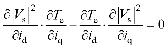
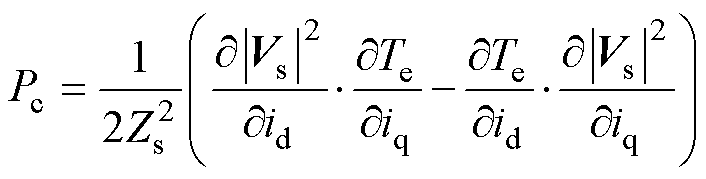
where 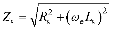 ; Pc is the defined MTPV penalty function.
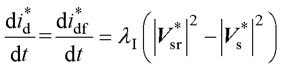
By substituting Equ.(1), Equ.(2) into Equ.(5) and ignoring the inductive voltage on the inductances at steady state, Equ.(5) can be modified as
 (6)
(6)
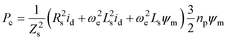
Then, Equ.(6) can be re-arranged as
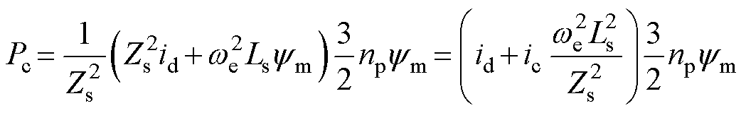 (7)
(7)
Since  is a penalty function and
 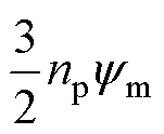 can be regarded as a constant gain, it will not influence the MTPV calculation, the MTPV penalty functionPc can be further derived as
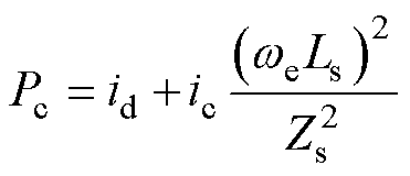 (8)
(8)
where ic is the machine characteristic current, i.e. ym/Ls.
Since the MTPV controller aims to generate the proper current command trajectory, id in Pc can be replaced by the d-axis current command . There- fore, the penalty function can be revised to

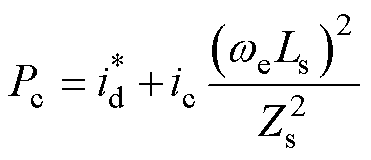 (9)
(9)
In this paper, Pcin Equ.(9) is finally selected as the MTPV penalty function for both DQFFC and CAAFFC. The two flux-weakening methods are detailed as follows.
1)DQFFC
For the DQFFC, as shown in Fig.4a, the initial d- and q-axis current commands, i.e.  and
and  , are obtained by considering MTPA in region Ⅰ, i.e. =0,
  . In the flux-weakening region, the initial d- and q-axis current commands are further modified by DCVFC and MTPV controller, respectively, according to Equ.(10) and Equ.(12) as follows.
According to part Ⅰ of Fig.4a, DCVFC[15, 18-19] can be expressed as
 (10)
(10)
where  is the integral gain of DCVFC;
  is the demagnetizing d-axis current command;
  is the voltage magnitude reference which can be set at
  , where M is the coefficient that can be used to adjust the voltage magnitude reference. When M≤1, the system operates in the linear modulation region. For the MPEOM, when
  , the voltage magnitude can be extended to the hexagon boun- dary[41].
As shown in part Ⅱ of Fig.4a, the MTPV controller for DQFFC can be expressed as
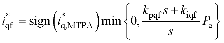 (11)
(11)
where kpqfand kiqfare the proportional and integral gains of the PI controller, respectively;  is the output of the MTPV controller.
Therefore, the q-axis current command can be finally obtained as
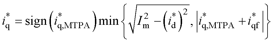 (12)
(12)
2) CAAFFC
For the CAAFFC, as shown in Fig.4b, con- sidering the MTPA in region Ⅰ, the initial lead angle of the current vector with respect to q-axis is zero, the current amplitude  is obtained from the speed controller. In the flux-weakening region, the initial current lead angle and amplitude are modified by CAVFC and MTPV controller, respectively, according to Equ.(13) and Equ.(15) as follows. According to the part Ⅰ of Fig.4b, CAVFC[20-23] can be expressed as
 (13)
(13)
where is the integral gain of CAVFC;
  is the lead angle of the current vector with respect to the q-axis.
As shown the part Ⅱ in Fig.4b, the MTPV controller for the CAAFFC can be expressed as
 (14)
(14)
where is the integral gain of the MTPV con- troller;
  is the output of the MTPV controller.
Therefore, the current amplitude can be finally obtained as
 (15)
(15)
where  is the modified current amplitude.
It should be noted that MTPV controller in DQFFC is a PI controller while the MTPV controller in CAAFFC is a pure integral controller. The difference between the two MTPV controllers will be further addressed in section Ⅲ.
In the flux-weakening region, considering the small signal behavior of the current command trajectory regulation, the operation modes considering the MTPV control can be distinguished by Modes A, B, C, and D. In Mode A, the current command is regulated along the current circle with a specific radius. In Mode B, the current trajectory is regulated along the constant torque curve. In Mode C, the current trajectory is regulated along the MTPV curve. In Mode D, the current trajectory is regulated along the normal direction of the current circle. Fig.5 illustrates the operation modes of DQFFC and CAAFFC. For the DQFFC, as shown in Fig.4a, the operation modes include Modes A, B, and C. For CAAFFC, as shown in Fig.4b, the operation modes include Modes A and D.
In region Ⅱ, no MTPV controller is required, only the voltage feedback controllers, i.e. DCVFC and CAVFC, are activated. Therefore, the voltage loop can be analyzed firstly under Modes A and B without considering MTPV controller. Subsequently, the MTPV loops of the two methods are analyzed in region Ⅲ.
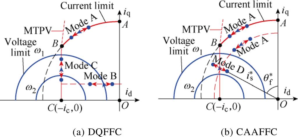
Fig.5 Operation modes in the flux-weakening region
In order to generalize the analysis of the voltage loop with DCVFC and CAVFC, the expression of CAVFC can be transformed into the equivalent form as DCVFC by using the following relationship
 (16)
(16)
where the variable with superscript ‘0’ denotes the corresponding value on the equilibrium point. By substituting Equ.(16) into Equ.(13), the expression of CAVFC can be derived as
 (17)
(17)
Therefore, the equivalent block diagram of the linearized voltage loop with DCVFC and CAVFC can be both depicted in Fig.6.
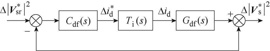
Fig.6 Linearized model of voltage loop
In Fig.6,  , Ti(s), and
  are the transfer functions of the integral controller, the equivalent current loop, and the control plant, respectively. Therefore, can be expressed as
 (18)
(18)
where  is
is
 (19)
(19)
Ti(s) can be expressed as
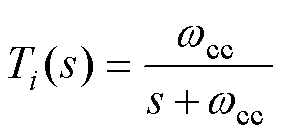 (20)
(20)
where  is the bandwidth of the current loop.
can be expressed as
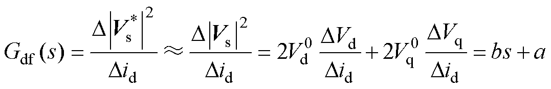 (21)
(21)
Under the assumption that the machine’s mechanical time constant is much greater than the electrical time constant, the variation of the machine speed is ignored at the equilibrium point. Assuming that  =
= , a and b can be derived as
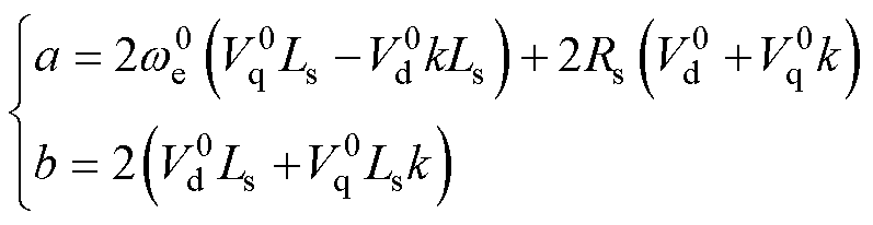 (22)
(22)
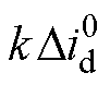
where the coefficient k in Modes A and B can be obtained as
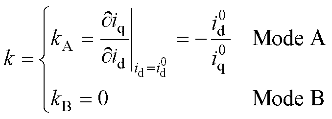 (23)
(23)
Therefore, the closed-loop transfer function of the voltage loop with DCVFC and CAVFC, i.e.  and
and  can be expressed as
 (24)
(24)
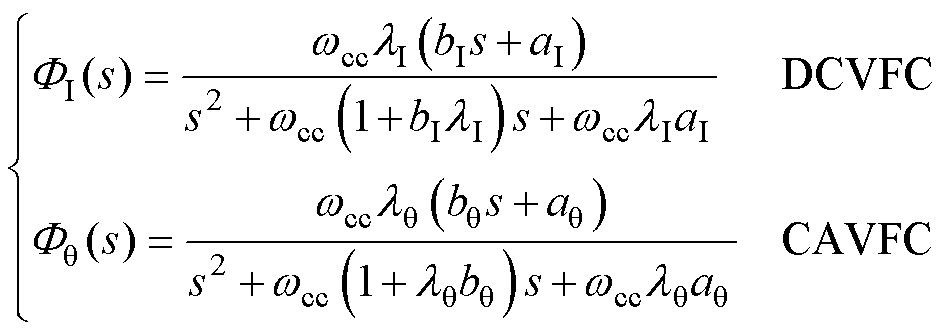
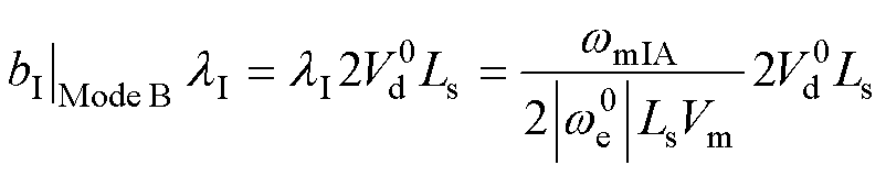
wherebI=b, aI=a;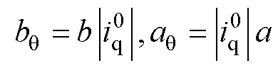 .
.
According to Routh stability criterion and Equ.(24), the stability of the voltage loop requires that
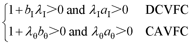 (25)
(25)
Since the negative d-axis current is required for the flux-weakening control, the control parameters and  are normally set at positive values. In addition, the conditions
 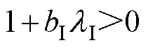 and
and  can be satisfied with the properly tuned control parameter (Appendix B). Therefore, the condition aI≤0 and
  ≤0, i.e. a≤0 defines the inherently unstable area of the voltage loop.Based on the machine parameters in Appendix A, when
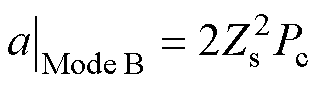
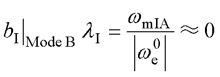
  , the map of the coefficients a in the Modes A and B can be illustrated in Fig.7, which are denoted asa|Mode A and a|Mode B, respectively. It can be seen that both Modes A and B have unstable areas, i.e. where a≤0.
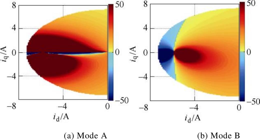
Fig.7 Map of coefficient a under different operation modes
To be more specific, in Mode A, at the equili- brium point, the coefficients a can be derived as
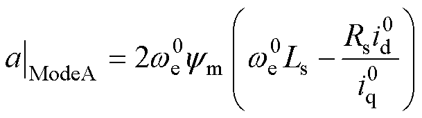
 (26)
(26)
Since 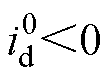 in the flux-weakening region, Equ.(26) implies that a|Mode A≤0 only occurs when
 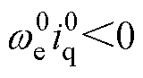 and
and 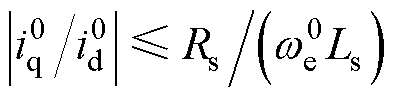 . Therefore, in Mode A, the instability happens at light load in generating condition, which is located at the lower half part of the current plane, as shown in Fig.7a. According to the operation mode definition of the two flux-weakening methods, this unstable condition can occur in CAAFFC.
In the Mode B (k=0), the coefficients a can be derived as
 (27)
(27)
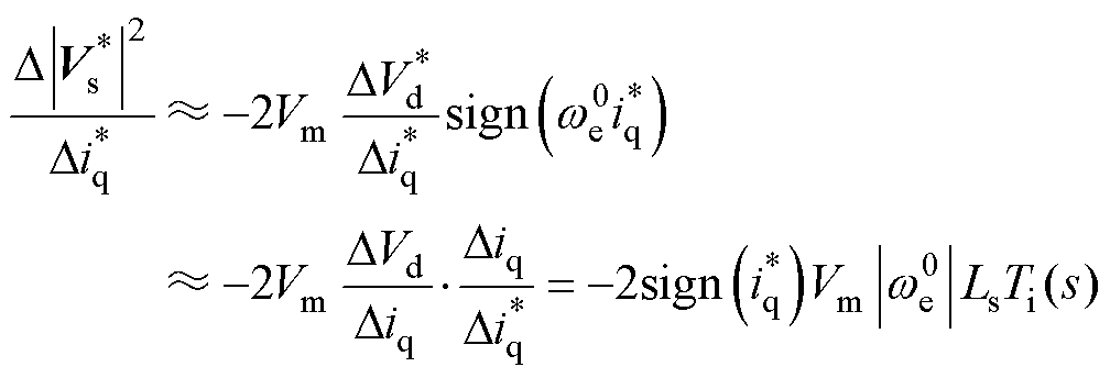
Therefore, a|Mode B=0 also defines the MTPV curve. As shown in Fig.7b, in Mode B, only the right part of the MPTV curve where a|Mode B>0 can allow a stable voltage control. Since when a|Mode B=0, the MTPV controller will be activated, the system will transfer to Mode C (region Ⅲ), the stability of the DQFFC can be maintained by the properly designed MTPV controller as will be discussed in the following section. However, there still exists a region where a|Mode B is positive but very close to zero, which is close to and on the right side of the MTPV curve. This area implies the weak voltage regulation capability of the voltage loop in DQFFC. The system in this area is in a fragile state and could easily oscillate especially in the over modulation region due to the reduced voltage margin and the increased harmonics. Although the VVM can Boost the current dynamics in the over modulation region, it cannot improve the voltage regulation capability reflected by the coefficient a, which is operation point relevant. This phenomenon will be further demonstrated in the experimental part. On the contrary, CAAFFC shows an advantage when the system approaches MTPV curve due to the large coefficient a in Mode A, which indicates that the voltage loop in CAAFFC is stable in region Ⅲ even without MTPV control.
The voltage regulation capability at different regions under Modes A and B can also be illustrated in Fig.8. In Fig.8, the label ‘A1’ represents the region which is close to the MTPV curve, the label ‘A2’ represents the region which is at light load in the generation condition. In Fig.8a and Fig.8b, at region ‘A1’ in Mode A and the region ‘A2’ in Mode B, the current regulation direction tends to be perpendicular to the voltage limit circle. However, at region ‘A2’ in Mode A and the region ‘A1’ in Mode B, the current regulation direction tends to be tangent to the voltage limit circle, in which condition the voltage feedback controller tries to move the operation point to the outside of the voltage limit circle at both regulation directions, implying that the voltage feedback controller loses its voltage regulation capability which could lead to oscillation or even instability.
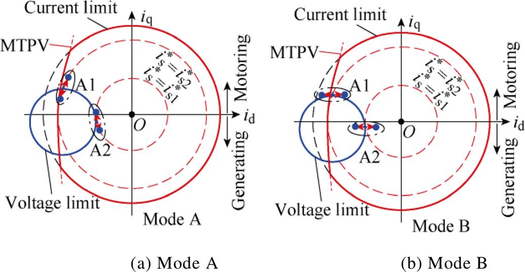
Fig.8 Voltage regulation illustration in different modes ( )
)
Based on the above analysis, the voltage regulation capabilities for CAAFFC and DAAFFC can be further illustrated from the control aspect of d- and q-axis currents. For CAAFFC in Mode A, Fig.9a, it can be regarded as mainly q-axis current control. For CAAFFC, in region A1, the q-axis current control is stable by regulating the current inside the voltage limit circle. While in region A2, the q-axis current control is unstable since the current cannot be regulated inside the voltage limit circle. For DQFFC in Mode B, Fig.9b, it is mainly d-axis current control. For DQFFC, the d-axis current control is unstable in region A1 and becomes stable in region A2. Overall, in Fig.9c, to obtain a stable operation, in region A1, q-axis current control should be employed while d-axis current control should be employed in region A2.

Fig.9 Voltage regulation illustration with different flux-weakening control methods
Besides, since the two flux-weakening methods are regulated in two different coordinate systems, CAAFFC has poor transition performance between motoring and generating condition. As shown in Fig.10a, for CAAFFC, when the system tries to transfer from the motoring condition to generating condition, e.g. from point F1to F4, as the speed controller can only regulate the current amplitude, the current command trajectory has to shrink to the original point first. Therefore, it will pass a region, e.g. the point F2in Fig.10a, which is outside of the voltage limit circle. The point F2 is unstable since the CAVFC tries to regulate it to the point F3, which is still outside of the voltage limit circle. Therefore, the transition between the motoring and generating conditions requires passing an unstable area, which deteriorates the system performance, especially at a light load condition. However, for DQFFC, as shown in Fig.10b, the system can smoothly transfer from F1 to F4 due to that the transition points F2 and F3 are all stable.
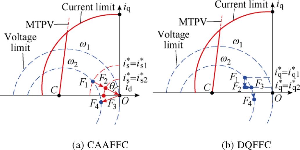
Fig.10 Transition from motoring to generating condition
In region Ⅲ, the system is regulated by both the MTPV controller and the voltage feedback controller, the operation Mode B or A activated by DCVFC and CAVFC cooperates with the Mode C or Mode D activated by the MTPV controllers in DQFFC and CAAFFC, respectively. Due to the different operation modes in DQFFC and CAAFFC, the MTPV controller design exhibits some differences, which will be discussed as follows.
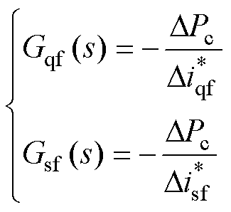
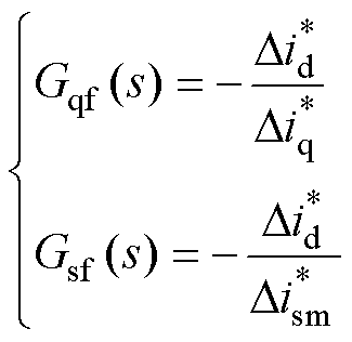
The linearized block diagram of the MPTV loop in DQFFC and CAAFFC can be shown in Fig.11a and Fig.11b, respectively. In Fig.11,Cqf(s) and Csf(s) are the transfer functions of the MTPV controller in DQFFC and CAAFFC, respectively; Gqf(s) and Gsf(s) are the transfer functions of the control plant of the MTPV loop in DQFFC and CAAFFC, respectively; δ is the assumed reference, which is an infinitesimal value. Gqf(s) and Gsf(s) can be obtained as
 (28)
(28)
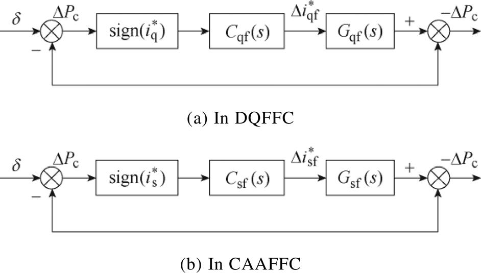
Fig.11 Linearized model of the MTPV Loop
It is reasonable to assume that the speed loop is much slower than the MTPV loop. Therefore,at the equilibrium point,  and
and  can be approxi- mated as
  and
and  , respectively. According to Equ.(7), ∆Pc can be approximated to
  . Therefore, Gqf(s) and Gsf(s) can be rewritten as
 (29)
(29)
The corresponding MTPV controllers in DQFFC and CAAFFC can be designed separately as follows.
1) MTPV Controller Design in DQFFC
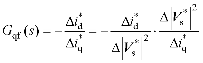
Since cannot directly induce, and comes from DCVFC, Gqf(s) can be reconstructed as
 (30)
(30)
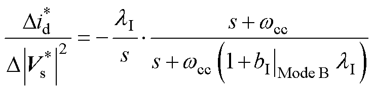
Due to that a|Mode B=0 in region Ⅲ,the term 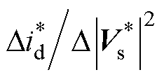 in Equ.(30) can be derived according to Fig.6, which can be written as
 (31)
(31)
According to Appendix section 2,  can be expressed as
 (32)
(32)
In region Ⅲ,  , and
, and  is very small, Hence, can be approximated as zero which is expressed as
 (33)
(33)
Therefore, can be derived that
 (34)
(34)
In addition, it has
 (35)
(35)
In region Ⅲ,  is close to zero and
 due to that
  . Therefore, it can be
derived that
 (36)
(36)
Consequently, the control plant of the MTPV loop in DQFFC can be derived as
 (37)
(37)
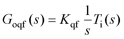
where Goqf(s) is the open-loop transfer function of the MTPV loop in DQFFC;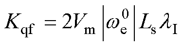 .
.
Equ.(35) explains that a pure integral controller is not applicable for the MTPV controller in DQFFC, as the system could oscillate due to the resultant origin pole of the closed-loop transfer function. To maintain the stability in region Ⅲ for DQFFC, a PI controller can be adopted. It is reasonable to make a further simplification of Equ.(37) by approximating Ti(s) as a unity gain when the MTPV loop is tuned with a bandwidth much lower than the current bandwidth. Thus, the closed-loop function of the MTPV loop can be obtained as
 (38)
(38)
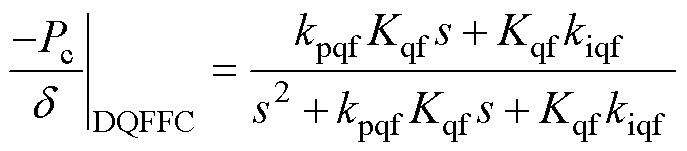
As a second-order system, the control parameters can be tuned as
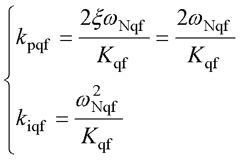 (39)
(39)
where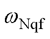 is the selected natural frequency,
  is the selected damping factor which can be set at 1.
2) MTPV Controller Design in CAAFFC
According to the foregoing analysis, the voltage loop in CAAFFC is stable in region Ⅲ, and can induce directly, 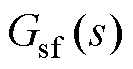 can be derived as
 (40)
(40)
It can be seen that the control plant is only a proportional gain. Therefore, a pure integral controller is enough. In addition, in region Ⅲ,  and
and  . For a conservative design, the controller can be tuned when =
 . Therefore, the closed-loop transfer function of the MTPV loop in CAAFFC can be derived as
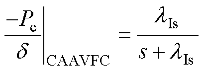 (41)
(41)
where  is the integral gain, which can be appro- ximated as the bandwidth of the MTPV loop.
The experiments based on the dSPACE platform are implemented on a non-salient PMSM. The power switches of the inverter are IRFH7440 MOSFET. The PWM switching frequency is 10 kHz. The load torque is provided by a wound field excited DC machine with a rated power of 150 W and a rated speed at 4 000 r/min. The combined inertia of the transmission system is 0.001 kg·m2. The machine and drive parameters are listed in Appendix section 1. The overall test rig is shown in Fig.12.
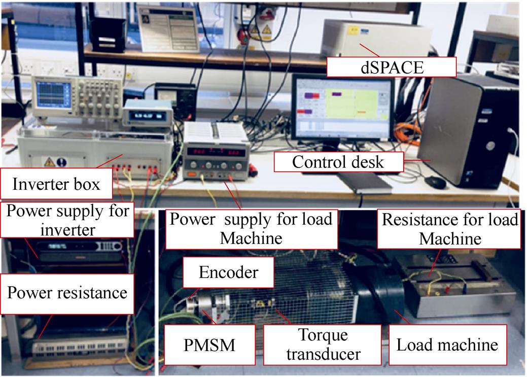
Fig.12 Overall test rig
In the experiments, the stability of the voltage loop in DQFFC and CAAFFC when the systems approach and pass through the MTPV curve is firstly demonstrated by enabling and disabling the MTPV controller. Subsequently, using MTPV controller, the performance when the systems approach the MTVP curve is compared between the two flux-weakening methods in both linear and over modulation regions. Finally, the transition performances of the two flux- weakening methods between motoring and generating conditions are demonstrated.
When M=0.9, for a given speed command n*= 1 500 r/min with the speed ramp at 750 r/min/s, Fig.13 shows the system performance with and without MTPV controller in DQFFC. In Fig.13a, without MPTV controller, it can be seen that the system cannot stabilize on the MTPV curve (Pc=0). In addition, the voltage  shows a short untracked period after Pc passes through zero. Fig.13b shows that the system is stable on the MTPV curve (Pc=0) with the PI MPTV controller, and the machine can achieve a higher speed than the system without MTPV controller. In contrast, Fig.14a shows the signal waveform in CAAFFC without MTPV controller. It can be seen that the voltage is well tracked even after Pc passes through zero without MTPV controller in CAAFFC. Fig.14b shows that the system can stabilize on the MTPV curve when an integral MTPV controller is applied, and thus the machine can achieve a higher speed.
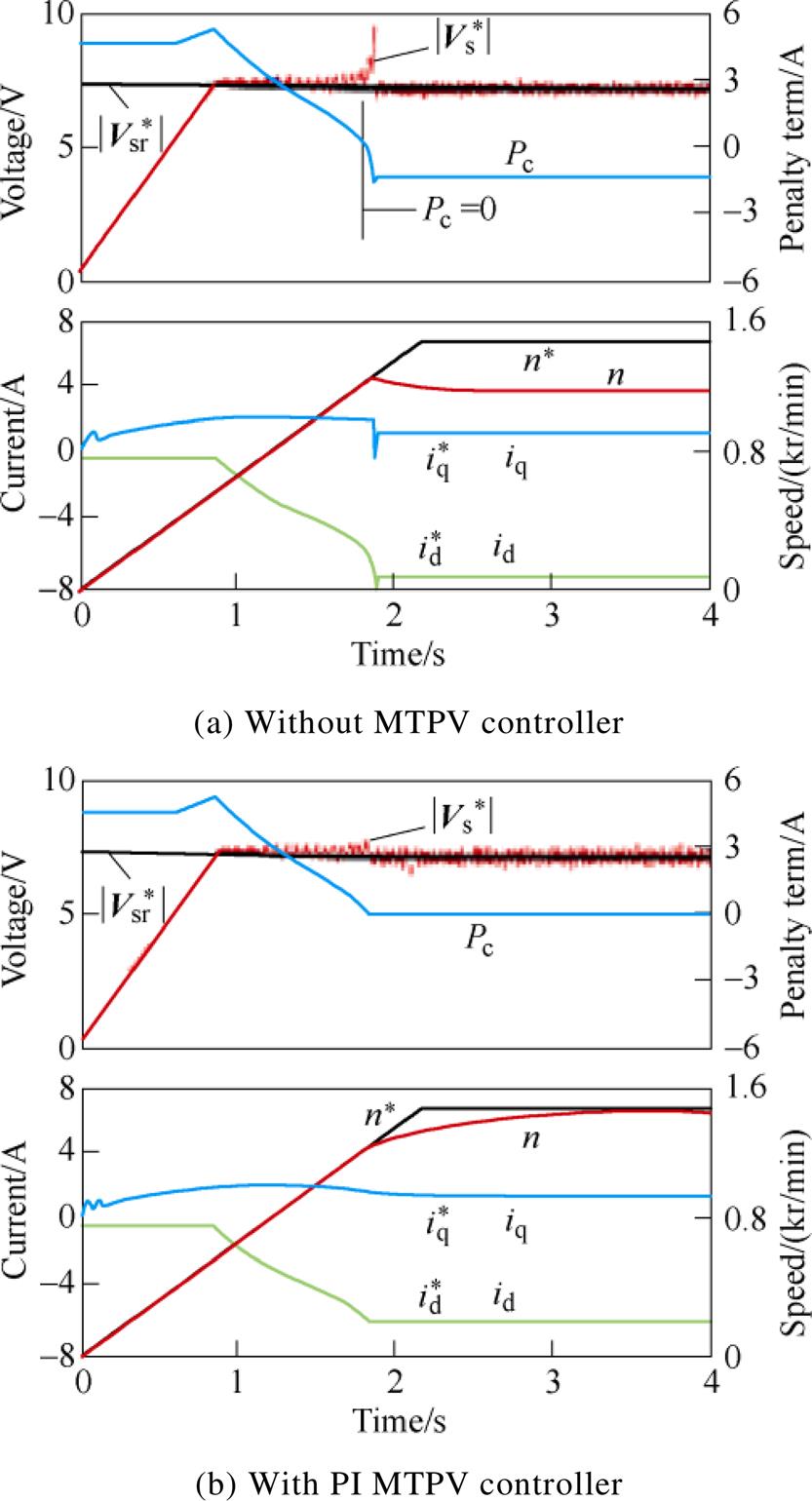
Fig.13 System performance of DQFFC
Meanwhile, the current trajectories with and without MTPV controller in DQFFC and CAAFFC are shown in Fig.15 and Fig.16, respectively.
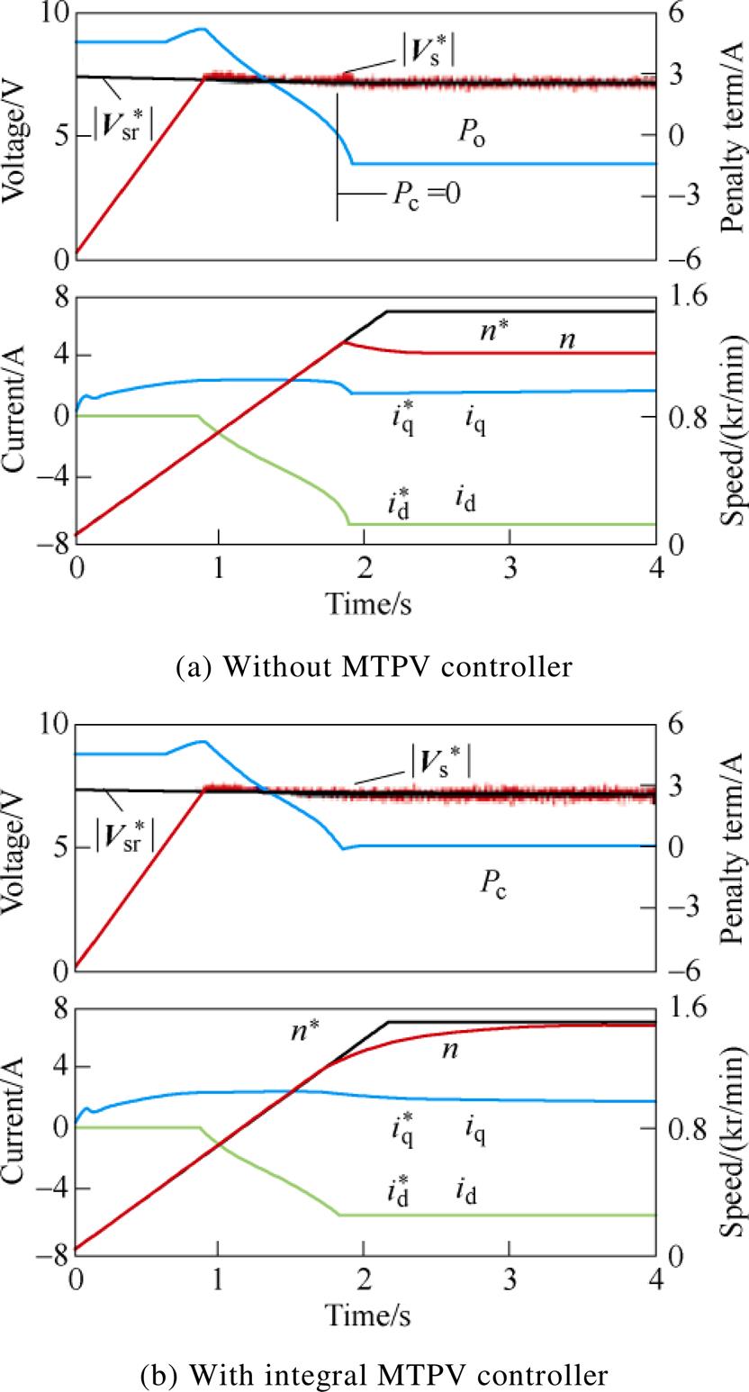
Fig.14 System performance of CAAFFC
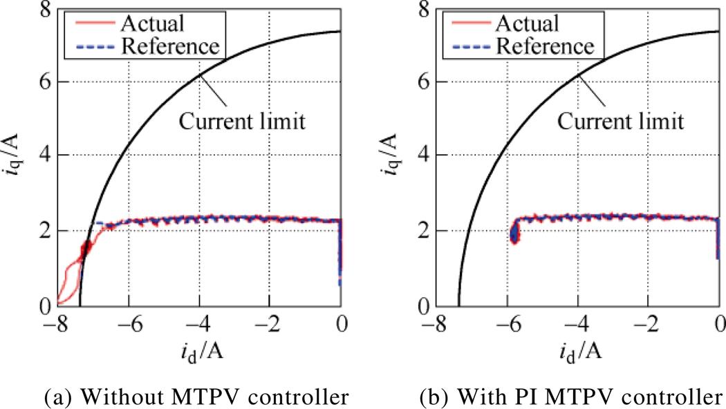
Fig.15 Current trajectory of system with DQFFC
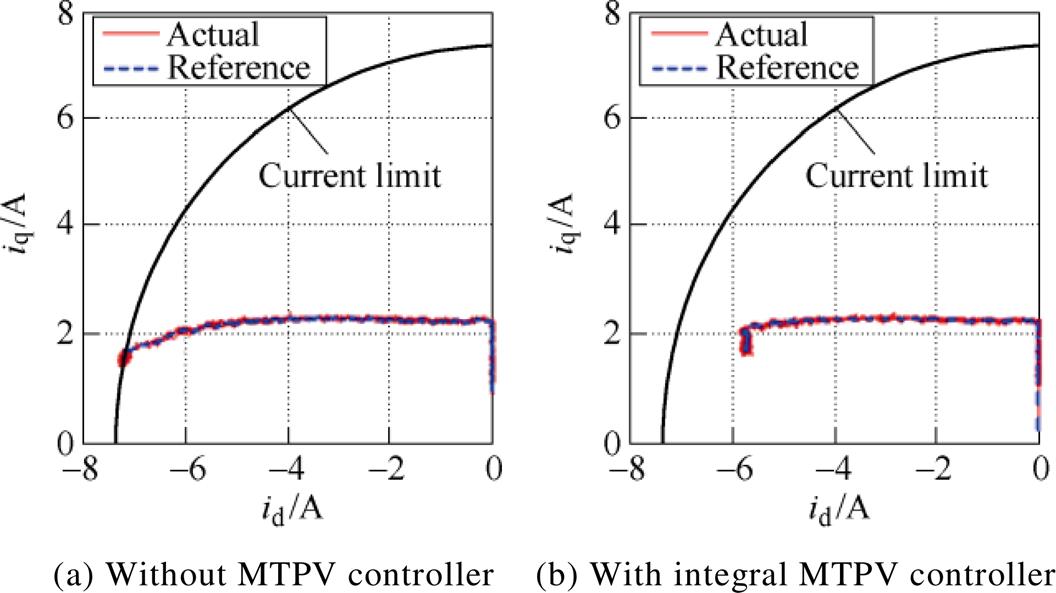
Fig.16 Current trajectory of system with CAAFFC
For the DQFFC without MTPV controller, it can be seen from Fig.15a that the current cannot be tracked well after the system passes through the MTPV curve, and the system is finally stabilized on the current limit. Fig.15b shows the well tracked current trajectory after the applied MTPV controller, and the system is finally stabilized on the MTPV curve. For the CAAFFC without MTPV controller, it can be seen from Fig.16a that the current can be tracked well even after the system passes through the MTPV curve, and the system is also stabilized on the current limit. In Fig.16b, it indicates that the MTPV loop is still required to force the system to operate on the MTPV curve for CAAFFC.
It should be noted that an integral MTPV controller in DQFFC cannot maintain system stability in region Ⅲ, which is shown in Fig.17.
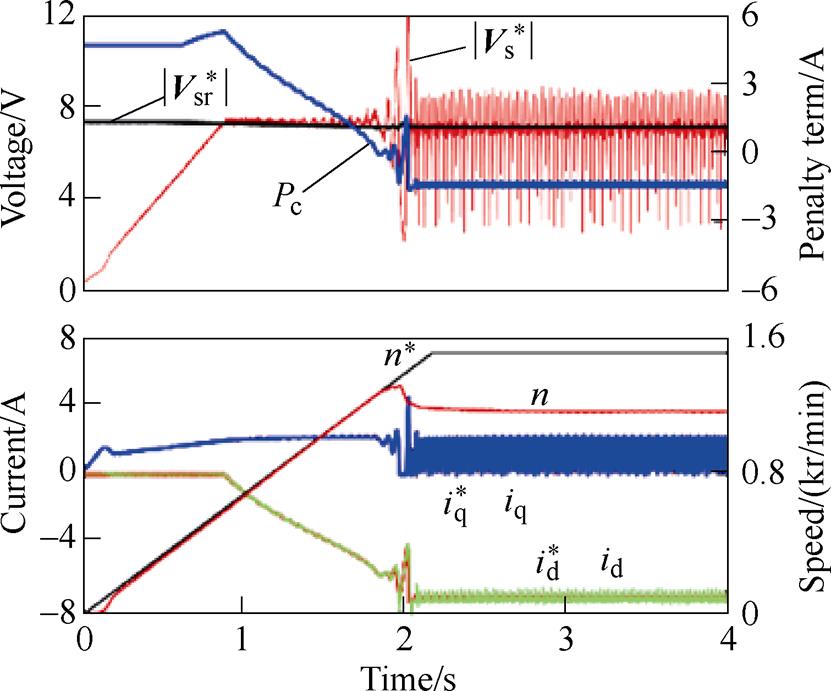
Fig.17 System performance of DQFFC with an integral MTPV controller
Therefore, in the current limit circle, it confirms that the MTPV curve defines the stable boundary of the voltage loop in DQFFC. The voltage loop in DQFFC loses control after the system passes MTPV curve. The stability of DQFFC in region Ⅲ can be guaranteed with a PI MTPV controller. Although the voltage loop in CAAFFC is stable even after the system passes MTPV curve, the MTPV controller is still required to force the system to operate on the MTPV curve.
With the applied MTPV controller, the perfor- mance when the systems approach MTPV curve is observed by changing the speed command from 0 r/min to 600 r/min, 700 r/min, 800 r/min, 900 r/min and 1 000 r/min every 2 s. Fig.18 shows the system performance of the two flux-weakening methods in the linear modulation region and M=0.9. As shown in Fig.18, although a short voltage pulse appears when approaching the MTPV curve for DQFFC, overall, the systems perform well for the two flux-weakening methods.
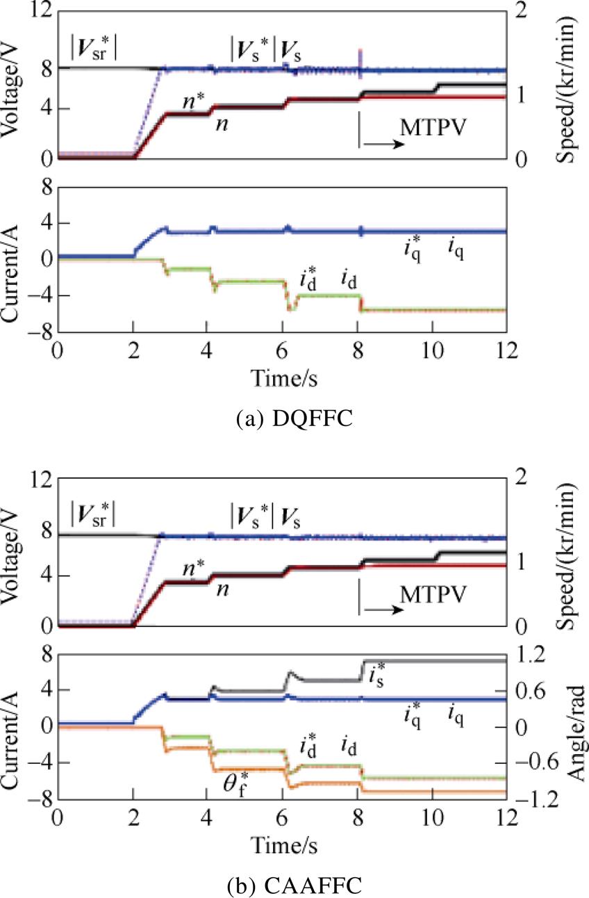
Fig.18 System performance when approaching MTPV curves without VVM (M=0.9)
Fig.19 shows the system performance without VVM in the over modulation region and M=1.15. It can be seen from Fig.19a that the system with DQFFC oscillates seriously in the flux-weakening region. In Fig.19b, the CAAFFC in the flux-weakening region is not as serious as DQFFC. However, the ripples in both current and voltage are much higher than those in the linear modulation region.

Fig.19 System performance when approaching MTPV curves without VVM (M=1.15)
Fig.20 shows the system performance with VVM when M=1.15. It can be seen from Fig.20a that the oscillation in DQFFC disappears on the MTPV curve and when the system is not close to MTPV curve. However, the oscillation still appears when the system gets closer to the MTPV curve. In Fig.20b, no oscillation occurs when the VVM is employed for CAAFFC. It should be noted that the voltage ripple in |Vs| is caused by the MPEOM block. The frequency of the ripple in |Vs| is six times the fundamental frequency.
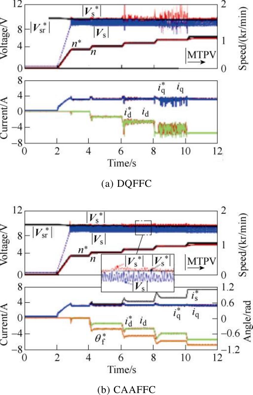
Fig.20 System performance when approaching MTPV curves with VVM (M=1.15)
Therefore, when approaching the MTPV curve, the CAAFFC shows better stability than the DQFFC especially in the over modulation region.
Fig.21 shows the transition performance of the two flux-weakening methods with the speed command n*=1 200 r/min and when M=0.9. The load torque is regulated manually by changing the exciting current of the DC machine. It can be seen from Fig.21a that the system with DQFFC can stably and smoothly transfer between motoring and generating conditions. However, as shown in Fig.21b, the system with CAAFFC cannot stably transfer between motoring and generating conditions. In addition, the current oscillates and the voltage loop loses control when the system tries to operate at the light load and generating condition in CAAFFC, which confirms the foregoing analyses.
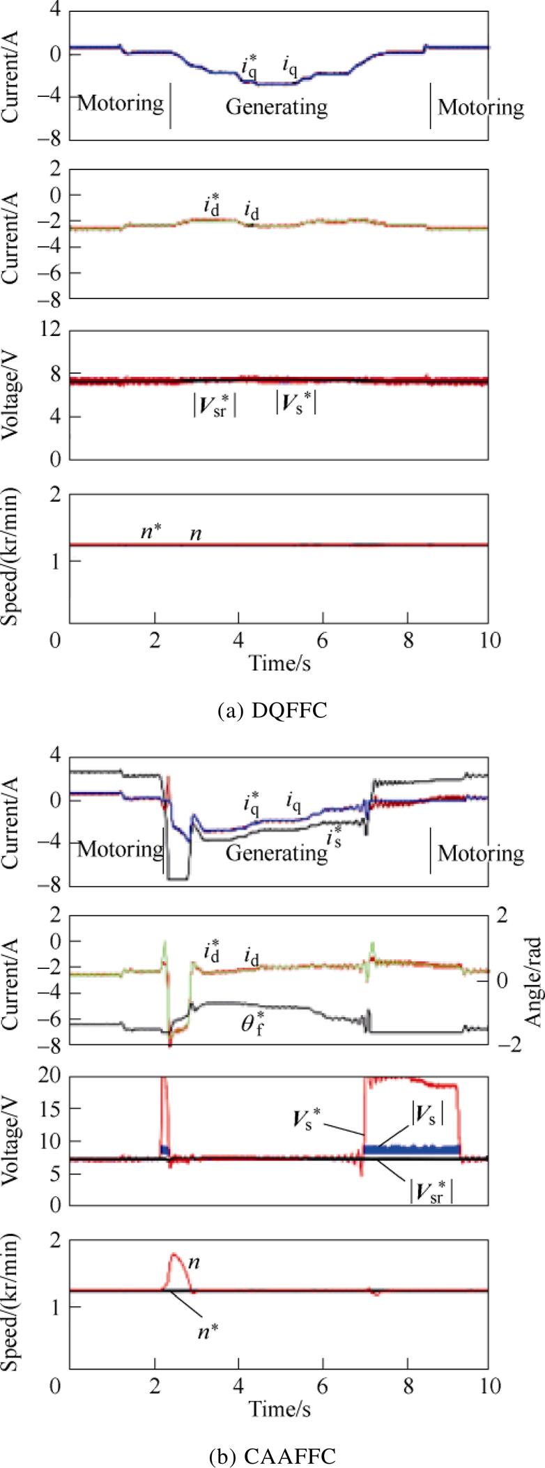
Fig.21 Transition performance between motoring and generating conditions
Based on the two conventional voltage feedback controllers, i.e. DCVFC and CAVFC, by further considering the MTPV control, this paper has comparatively studied the stability of the two flux- weakening methods, i.e. DQFFC and CAAFFC, based on a non-salient PMSM. The feedback type MTPV controllers in DQFFC and CAAFFC are analyzed and designed.
The analyses and experimental results have indicated that apart from the control parameters, DQFFC and CAAFC have instability issues inherently. The instabilities can be different between these methods in two different operation regions:
1) When approaching MTPV curve, the DQFFC method has a weak voltage regulation capability, since only d-axis current can be regulated, which prevents the current from moving inside the voltage limit circle. This could lead to oscillation in over modulation. On the other hand, CAAFFC mainly regulates the q-axis current, allowing the current to move within the circle. Thus, the oscillation can be alleviated.
2) When the machine operates under a light load, the CAAFFC with q-axis current regulation has instability issues which cause an unstable transition between motoring and generating modes. On the other hand, DQFFC with d-axis current regulation has no issues and can achieve a smooth and stable transition.
Appendix
1. Machine and drive parameters
App.Tab.1 Machine and drive parameters
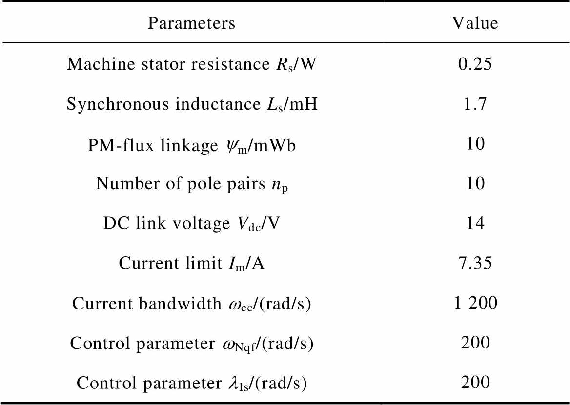
ParametersValue Machine stator resistance Rs/W0.25 Synchronous inductance Ls/mH1.7 PM-flux linkage ym/mWb10 Number of pole pairs np10 DC link voltage Vdc/V14 Current limit Im/A7.35 Current bandwidth wcc/(rad/s)1 200 Control parameter wNqf/(rad/s)200 Control parameter lIs/(rad/s)200
2. Control parameter design of voltage feedback con- trollers
According to Equ.(24), the characteristic equation of the closed-loop transfer function with DCVFC and CAVFC, qI(s) and qq(s) can be expressed as
 (A1)
(A1)
where blI=bIlI;alI=aIlI; blq=bqlq; alq=aqlq.
For the controller design in the flux-weakening region, the voltage drop on resistance can be ignored. According to the different operation modes, and the coefficients blI, alI, blq and alqcan be further derived as
 (A2)
(A2)
 (A3)
(A3)
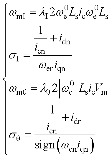
where wb=Vm/(LsIm); Vdn is  normalized by Vm;wmI, wmq, sI and sqcan be expressed as
 (A4)
(A4)
where idn and iqn are and
and  normalized by Im, respectively; icn is ic normalized by Im; wen is
  norma- lized by wb; sI and sq can be seen as the non-dimensional coefficients which vary with the operation points.
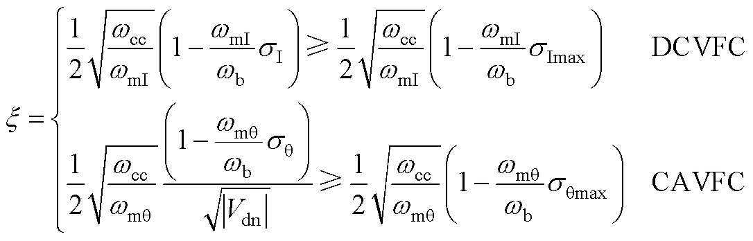
Therefore, the proper lI and lq can be obtained with the proper wmI and wmq. In Mode A, according to Equ.(A1)~Equ.(A3), the damping factors for the voltage loop with DCVFC and CAVFC satisfy the following relationships
 (A5)
(A5)
where sImax and sqmaxdenote the maximum value of sIand sqin the flux-weakening region. If the system is designed when sI=sImax and sq=sqmax, wmI and wmqcan be solved as
 (A6)
(A6)
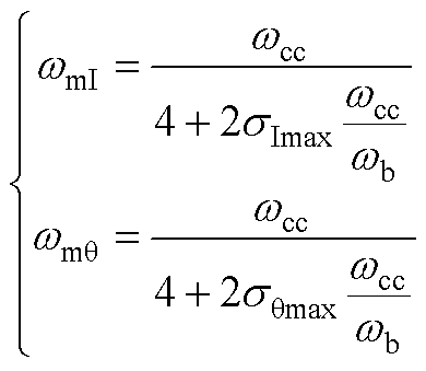
As a conservative design, wmIand wmqcan be simplified to their lower boundary. For the critical damping condition, i.e.  =1,the simplified wmIand wmq can be obtained as
 (A7)
(A7)
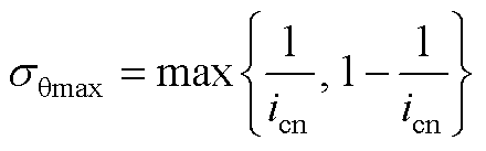
According to Equ.(A4), sqmax can be obtained as
 (A8)
(A8)
Therefore, the control parameter of CAVFC can be tuned as
 (A9)
(A9)
For the DCVFC, since sImaxcould be positive infinity when idn=-1 and iqn=0, the control parameter lI should be theoretically zero, which is not practical. Fig.22 shows the variation of sI when icn=0.8 (for the machine in this paper) in Mode A. As can be seen from Fig.22, the extreme condition, i.e. when idn=-1, can be reasonably ignored as the system will transfer to Mode C when idn=-0.8. Therefore, sImax can be set at a value, which is higher than most of the operation points except the region where idnapproaches -1. According to Fig.22, in this paper, sImax is set at 2. When ξ=1, the control parameter of DCVFC in Mode A can be tuned as
 (A10)
(A10)
where  .
.
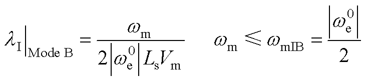
In Mode B, since the Routh stable criterion requires that 1+blI|Mode B>0 and alI|Mode B>0, the worst condition happens when is minimum, i.e.  , which defines the minimum stable range for the control parameter lI.
Assuming that lIis tuned so that 1+blI|Mode B>0.5 at the worst condition, the control parameter lIin the Mode B can be set as
 (A11)
(A11)
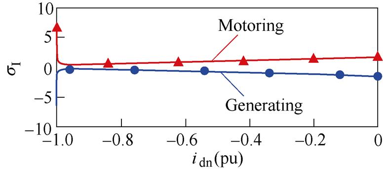
App.Fig.1 Variation of sI against idn when icn=0.8 in Mode A
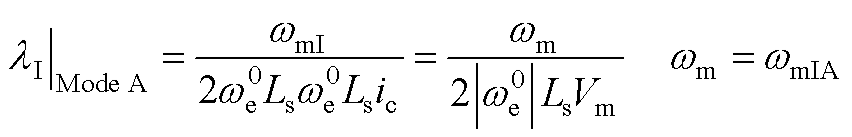
In addition, it should be noted that wmIA is obtained in Mode A and is inversely proportional to the machine speed. When the system transfers to Mode C, wmIA will be too small if the machine speed goes too high. Therefore, the minimum wmIA can be obtained at the point when the system transfers to Mode C, and itcan be approximately obtained when idn=-icn, i.e. wmI/1.3 for icn=0.8. Therefore, by considering Mode C, wmIA can be further revised as
 (A12)
(A12)
Finally, the control parameter lI can be set as
 (A13)
(A13)
Since the MTPV controller is tuned in region Ⅲ, where wmIA is much smaller thanwmIB, bI|Mode BlIcan be approximated as zero for the MTPV controller design.
Reference
[1] Zhu Z Q, Howe D. Electrical machines and drives for electric, hybrid, and fuel cell vehicles[J]. Proceedings of the IEEE, 2007, 95(4): 746-765.
[2] Chau K T, Chan C C, Liu Chunhua. Overview of permanent-magnet brushless drives for electric and hybrid electric vehicles[J]. IEEE Transactions on Industrial Electronics, 2008, 55(6): 2246-2257.
[3] Villani M, Tursini M, Fabri G, et al. High reliability permanent magnet brushless motor drive for aircraft application[J]. IEEE Transactions on Industrial Elec- tronics, 2012, 59(5): 2073-2081.
[4] Giulii Capponi F, De Donato G, Del Ferraro L, et al. AC brushless drive with low-resolution Hall-effect sensors for surface-mounted PM Machines[J]. IEEE Transactions on Industry Applications, 2006, 42(2): 526-535.
[5] Soong W L. Field-weakening performance of brush- less synchronous AC motor drives[J]. IEE Proceedings- Electric Power Applications, 1994, 141(6): 331.
[6] EL-Refaie A M, Jahns T M. Optimal flux weakening in surface PM machines using fractional-slot con- centrated windings[J]. IEEE Transactions on Industry Applications, 2005, 41(3): 790-800.
[7] Morimoto S, Sanada M, Takeda Y. Wide-speed operation of interior permanent magnet synchronous motors with high-performance current regulator[J]. IEEE Transactions on Industry Applications, 1994, 30(4): 920-926.
[8] Tursini M, Chiricozzi E, Petrella R. Feedforward flux-weakening control of surface-mounted permanent- magnet synchronous motors accounting for resistive voltage drop[J]. IEEE Transactions on Industrial Electronics, 2010, 57(1): 440-448.
[9] Chen Y S, Zhu Z Q, Howe D. Influence of inaccura- cies in machine parameters on field-weakening performance of PM brushless AC drives[C]//IEEE International Electric Machines and Drives Con- ference,Seattle, WA, USA, 2002: 691-693.
[10] de Kock H W, Rix A J, Kamper M J. Optimal torque control of synchronous machines based on finite- element analysis[J]. IEEE Transactions on Industrial Electronics, 2010, 57(1): 413-419.
[11] Maric D S, Hiti S, Stancu C C, et al. Two flux weakening schemes for surface-mounted permanent- magnet synchronous drives. Design and transient response considerations[C]//Proceedings of the IEEE International Symposium on Industrial Electronics, Bled, Slovenia, 2002: 673-678.
[12] Nalepa R, Orlowska-Kowalska T. Optimum trajectory control of the current vector of a nonsalient-pole PMSM in the field-weakening region[J]. IEEE Transactions on Industrial Electronics, 2012, 59(7): 2867-2876.
[13] Zhu Z Q, Chen Y S, Howe D. Online optimal flux-weakening control of permanent-magnet brush- less AC drives[J]. IEEE Transactions on Industry Applications, 2000, 36(6): 1661-1668.
[14] Kim J M, Sul S K. Speed control of interior per- manent magnet synchronous motor drive for the flux weakening operation[J]. IEEE Transactions on Indu- stry Applications, 1997, 33(1): 43-48.
[15] Bianchi N, Bolognani S, Zigliotto M. High- performance PM synchronous motor drive for an electrical scooter[J]. IEEE Transactions on Industry Applications, 2001, 37(5): 1348-1355.
[16] Wang Chao, Zhu Z Q. Fuzzy logic speed control of permanent magnet synchronous machine and feedback voltage ripple reduction in flux-weakening operation region[J]. IEEE Transactions on Industry Appli- cations, 2020, 56(2): 1505-1517.
[17] Kwon Y C, Kim S, Sul S K. Six-step operation of PMSM with instantaneous current control[C]//2012 IEEE Energy Conversion Congress and Exposition (ECCE), Raleigh, NC, USA, 2012: 479-486.
[18] Bozhko S, Rashed M, Hill C I, et al. Flux-weakening control of electric starter-generator based on permanent- magnet machine[J]. IEEE Transactions on Transport- ation Electrification, 2017, 3(4): 864-877.
[19] Wang Chao, Zhu Z Q, Zhan Hanlin. Adaptive voltage feedback controllers on nonsalient permanent magnet synchronous machine[J]. IEEE Transactions on Indu- stry Applications, 2020, 56(2): 1529-1542.
[20] Miguel-Espinar C, Heredero-Peris D, Gross G, et al. Maximum torque per voltage flux-weakening strategy with speed limiter for PMSM drives[J]. IEEE Transa- ctions on Industrial Electronics, 2021, 68(10): 9254- 9264.
[21] Deng Tao, Su Zhenhua, Li Junying, et al. Advanced angle field weakening control strategy of permanent magnet synchronous motor[J]. IEEE Transactions on Vehicular Technology, 2019, 68(4): 3424-3435.
[22] Liu Qian, Hameyer K. A deep field weakening control for the PMSM applying a modified overmodulation strategy[C]//8th IET International Conference on Power Electronics, Machines and Drives (PEMD 2016), Glasgow, UK, 2016: 1-6.
[23] Bolognani S, Calligaro S, Petrella R. Adaptive flux- weakening controller for interior permanent magnet synchronous motor drives[J]. IEEE Journal of Emerging and Selected Topics in Power Electronics, 2014, 2(2): 236-248.
[24] Kwon T S, Sul S K. Novel anti-windup of a current regulator of a surface-mounted permanent-magnet motor for flux-weakening control[C]//Fourtieth IAS Annual Meeting. Conference Record of the 2005 Industry Applications Conference, Hong Kong, China, 2005: 1813-1819.
[25] Kwon Y C, Kim S, Sul S K. Voltage feedback current control scheme for improved transient performance of permanent magnet synchronous machine drives[J]. IEEE Transactions on Industrial Electronics, 2012, 59(9): 3373-3382.
[26] Liu Hesong, Zhu Z Q, Mohamed E, et al. Flux- weakening control of nonsalient pole PMSM having large winding inductance, accounting for resistive voltage drop and inverter nonlinearities[J]. IEEE Transactions on Power Electronics, 2012, 27(2): 942-952.
[27] Lin Pingyi, Lai Y S. Voltage control technique for the extension of DC-link voltage utilization of finite- speed SPMSM drives[J]. IEEE Transactions on Industrial Electronics, 2012, 59(9): 3392-3402.
[28] Zhang Yuan, Güven M K, Guven M K, et al. Experimental verification of deep field weakening operation of a 50-kW IPM machine by using single current regulator[J]. IEEE Transactions on Industry Applications, 2011, 47(1): 128-133.
[29] Zhu Lei, Wen Xuhui, Zhao Feng, et al. Deep field- weakening control of PMSMs for both motion and generation operation[C]//2011 International Conference on Electrical Machines and Systems, Beijing, China, 2011: 1-5.
[30] Miyajima T, Fujimoto H, Fujitsuna M. A precise model-based design of voltage phase controller for IPMSM[J]. IEEE Transactions on Power Electronics, 2013, 28(12): 5655-5664.
[31] Stojan D, Drevensek D, Plantic Ž, et al. Novel field-weakening control scheme for permanent- magnet synchronous machines based on voltage angle control[J]. IEEE Transactions on Industry Appli- cations, 2012, 48(6): 2390-2401.
[32] Bae B H, Patel N, Schulz S, et al. New field weakening technique for high saliency interior per- manent magnet motor[C]//38th IAS Annual Meeting on Conference Record of the Industry Applications Conference, Salt Lake City, UT, USA, 2004: 898-905.
[33] Choi G Y, Kwak M S, Kwon T S, et al. Novel flux-weakening control of an IPMSM for quasi six- step operation[C]//2007 IEEE Industry Applications Annual Meeting, New Orleans, LA, USA, 2007: 1315-1321.
[34] Cheng Bing, Tesch T R. Torque feedforward control technique for permanent-magnet synchronous motors[J]. IEEE Transactions on Industrial Electronics, 2010, 57(3): 969-974.
[35] Trancho E, Ibarra E, Arias A, et al. PM-assisted synchronous reluctance machine flux weakening control for EV and HEV applications[J]. IEEE Transactions on Industrial Electronics, 2018, 65(4): 2986-2995.
[36] Li Siyi, Su Jianyong, Yang Guijie. Flux weakening control strategy of permanent magnet synchronous motor based on active disturbance rejection control[J]. Transactions of China Electrotechnical Society, 2022, 37(23): 6135-6144.
[37] Li Xue, Chi Song, Liu Cong, et al. Flux-weakening control with single current regulator of permanent magnet synchronous motor based on virtual resistor[J]. Transactions of China Electrotechnical Society, 2020, 35(5): 1046-1054.
[38] Guo Jiaqiang, Liu Xu, Li Shanhu. Flux weakening control of variable flux reluctance machine con- sidering resistive voltage drops in armature and zero-sequence loop[J]. Transactions of China Electro- technical Society, 2021, 36(18): 3911-3921.
[39] Bao Xucong, Wang Xiaolin, Gu Cong, et al. Stability analysis and improvement design of current loop of ultra-high-speed permanent magnet motor drive system[J]. Transactions of China Electrotechnical Society, 2022, 37(10): 2469-2480.
[40] Song Xinxin, Zhao Wenxiang, Cheng Yu. Unity power factor field weakening control of field- modulated permanent magnet linear modulation motor with open winding[J]. Transactions of China Elec- trotechnical Society, 2021, 36(5): 893-901.
[41] Holtz J. Pulsewidth modulation-a survey[J]. IEEE Transactions on Industrial Electronics, 1992, 39(5): 410-420.
摘要 对于反馈式弱磁控制,通常有两种方法,即基于dq轴电流的反馈式弱磁控制(DQFFC)和基于电流幅值和角度的反馈式弱磁控制(CAAFFC),被广泛使用并被认为相互等价。该文基于最大扭矩电压比(MTPV)控制,对这两种方法的系统稳定性进行了比较研究。分析结果表明,不稳定既由控制参数设计引起,也与弱磁控制方法本身的特性有关。对于方法本身导致的不稳定,DQFFC和CAAFFC在不同的工作区域中表现出了不同的特性。基于在不同的工作区域内,该文从电流调节方向的角度来说明系统稳定和不稳定的工作机制。此外,针对DQFFC和CAAFFC在不同区域内的稳定性差异,给出了MTPV控制器的控制参数设计指南。最后,通过实验结果进行了演示和验证。
关键词:弱磁控制 不稳定 最大扭矩电压比 振荡 永磁同步电机 稳定性 电压反馈控制器
中图分类号: TM301.4
Received July 21, 2022;
Revised February 20, 2023.
DOI: 10.19595/j.cnki.1000-6753.tces.221398
Notes Brief
Wang Chao male, born in 1986, Advanced Research Engineer, Midea Welling Motor Technology Company, Ltd., Shanghai, China. Major research interests include the control of electric drives.E-mail: wangchao15@welling.com.cn
Zhu Z Q male, born in 1962, Fellow REng, Fellow IEEE, Fellow IET, PhD, Professor at the University of Sheffield, UK. Major research interests include design, control, and applications of brushless permanent magnet machines and drives for applications ranging from automotive through domestic appliances to renewable energy.E-mail: z.q.zhu@Sheffield.ac.uk (Corresponding author)
(编辑 崔文静)