 ),而磁场强度H为待求输出变量[8]。若在其中应用正磁滞模型,则会涉及复杂的迭代求解过程,从而造成电磁场数值计算更为耗时,甚至出现迭代不收敛等严重问 题[9-12]。而以磁通密度B为输入、磁场强度H为输出的逆磁滞模型则不存在该问题,因此其一直以来是国际电磁场领域研究的热点问题[7-12]。
摘要 如何在保证模拟精度的基础上,提升逆磁滞模型的计算速度一直以来是国际电磁场领域研究的热点问题。然而,现有所提逆磁滞模型难以兼顾精度与速度的双重要求。解析形式的逆磁滞模型具有较快的求解速度,如何提出高精度的此类模型是解决上述问题的关键所在。为此,该文利用课题组所提基于解析Everett函数推导而得的解析正Preisach磁滞模型,分别推导了初始磁化曲线、磁滞回线下降支与上升支的磁导率的解析表达式,继而利用差分法,推导得到了目前唯一一个解析的逆Preisach磁滞模型。通过对比仿真与实验结果,验证了所提解析逆Preisach磁滞模型的模拟精度,并在模拟精度与计算速度两方面将其与广泛应用的逆J-A磁滞模型进行对比,发现它的平均相对误差比逆J-A磁滞模型小10 %以上,且其计算速度约为逆J-A磁滞模型的2.67倍。
关键词:软磁材料 磁滞模型 解析逆Preisach模型
目前,取向及无取向硅钢等电工软磁材料已广泛应用于电机、变压器、电抗器等电工装备中[1-3]。然而,软磁材料本身固有复杂的非线性磁滞特性,其会对所属电工装备的能量损耗、电-磁-热多物理场、伏安关系等产生重要影响。因而如何准确模拟软磁材料的磁滞特性对电工装备的磁心损耗计算[4]、电磁暂态与多物理场仿真[5-6]、全局结构优化设计[7]等研究工作具有重要的支撑作用。随着智能电网、特高压输电、新能源发电等领域的快速发展,实际工程已对电工装备提出了更高要求,进而也对所用磁滞模型提出了更高要求:①模拟精度高;②求解速度快和能够高效解决大多数工程问题。传统的以磁场强度H为输入、磁通密度B为输出的正磁滞模型在实际应用中通常难以满足该要求[6]。因为在大多数涉及软磁材料的电工装备电磁场计算问题中,通常是以矢量磁位A作为求解变量,即内置磁滞模型的原始输入为磁通密度B(B=),而磁场强度H为待求输出变量[8]。若在其中应用正磁滞模型,则会涉及复杂的迭代求解过程,从而造成电磁场数值计算更为耗时,甚至出现迭代不收敛等严重问 题[9-12]。而以磁通密度B为输入、磁场强度H为输出的逆磁滞模型则不存在该问题,因此其一直以来是国际电磁场领域研究的热点问题[7-12]。
最早被提出的磁滞模型为基于磁滞算子假设的Preisach模型[13]。该模型通常相对其他磁滞模型而言,具有较高的模拟精度与普适性,因而得到了国内外学者广泛的关注与研究[10-19]。虽然经典Preisach模型为正模型,但目前已在其基础上发展了多种逆Preisach模型。然而,现有不同类型的逆Preisach模型存在如下问题:
(1)与经典Preisach模型类似的离散插值型逆Preisach模型[8, 10-11, 16]:待提取参数较多,且其提取过程复杂,同时在实际应用中较为不便与耗时。例如,文献[8]所提逆Preisach模型为提取参数,首先将Preisach分布函数取值域离散为密集的非均匀单元网格,继而利用多条实测磁滞回线提取与各网格对应的Preisach分布函数离散值。而后为模拟磁滞回线,需将磁通密度扫过的网格单元的面积提前通过插值法确定,而该过程通常需要人为手动处理。因而该类逆Preisach模型的参数辨识及其数值模拟过程较为复杂、繁琐与耗时,不利于磁滞回线的自动快速模拟,导致其与电工装备电磁多物理场数值计算、全局优化设计等研究的兼容性较差[6, 12]。
(2)基于逆Everett积分函数的离散插值型逆Preisach模型[6, 12, 15]:①不利于揭示与磁化过程相关的材料组分、结构和磁滞物理现象本质[18]。虽然利用实测磁滞回线可直接提取逆Everett函数离散值,进而避免经典Preisach模型复杂的双重积分运算,但逆Everett函数本质上是Preisach分布函数在特定区域的积分函数,而该积分处理会隐藏磁性材料内在的磁化特性与机制。通常而言,与磁化特性及机制直接相关的材料组分、结构等更清晰地反映在原始的Preisach分布函数上[20]。②通常只能在离散的逆Everett函数插值区域内求解磁场强度,而在插值区域以外则难以求解相应的磁场强度,从而限制了该类逆磁滞模型在实际工程中的应用。③在电工装备电磁场数值计算中,常涉及动态磁导率的求解[6, 19, 21],而为求解该磁导率,需对离散的逆Everett函数值作差分运算,但该操作会使实验误差进一步扩大,并且很可能还会因为插值得到的Everett函数不光滑而使求解的动态磁导率等参量不连续,继而导致相关电磁场计算出现不收敛的风险[18]。
(3)在经典Preisach模型基础上设置逆运算而得的数值迭代型逆Preisach模型[19, 22]:数值计算不稳定,且其求解时间较长。例如,文献[19]首先构建了一种基于实测极限磁滞回线下降支的正Preisach模型,而后对其求导得到磁通密度关于磁场强度的导数表达式,继而在给定初值的情况下,利用牛顿-拉夫逊法迭代求解未知的磁场强度。该类型的逆Preisach模型由于涉及非线性方程的迭代求解,故其数值计算过程并不稳定,且求解时间也较长。由于基于有限元等数值算法求解电工装备电磁多物理场本身已经较为耗时,若再引入此类磁滞模型,则将进一步增加系统的计算量。同时也增加了电工装备电磁多物理场计算不收敛的风险。
综上所述,提出高精度的解析逆Preisach模型(“解析”保证了相应模型具有较快的求解速度)是解决上述不同类型的逆Preisach模型所存问题的关键所在,且在电工装备的电磁多物理场仿真、电路系统全真模拟、全局结构优化设计等研究领域具有广阔的应用前景。然而,尚未见到解析逆Preisach模型的相关研究成果发表。
基于本课题组已提出的解析正Preisach模型[23],本文推导了不同类型磁滞回线段,即初始磁化曲线、磁滞回线下降支与上升支的磁导率的解析表达式。在此基础上,运用差分法推导出目前唯一一个属于解析形式的逆Preisach模型,并验证了该模型在取向及无取向硅钢等两类不同电工软磁材料中的模拟效果,另外也在精度与速度两方面与广泛应用的逆J-A磁滞模型进行了对比,证实了所提解析逆Preisach模型具备优异的综合性能。
经典Preisach理论认为磁性材料由大量具有矩形磁滞特性的磁偶极子组成,其宏观磁滞特性表现为全部磁偶极子磁滞特性的线性叠加[13]。经典Preisach模型属于标量正磁滞模型,以当前t时刻的磁场强度H(t)为输入、磁通密度B(t)为输出[16]。B(t)为
 (1)
(1)
式中, 为磁偶极子,取值为±1,具体由磁场强度的历史值与当前值共同决定;h1、h2分别为磁偶极子上升沿与下降沿的开关值;
 为磁偶极子的分布函数;S为Preisach分布函数的取值域。
由式(1)可知,经典Preisach模型包含了复杂的分布函数双重积分运算,而该运算会导致其模型参数辨识过程繁琐,计算时间较长,从而导致它的实用性大为降低。为此,有学者引入了Everett积分函数的概念。将Everett函数E(x, y)引入经典Preisach模型后,式(1)[19, 23]则可转变为
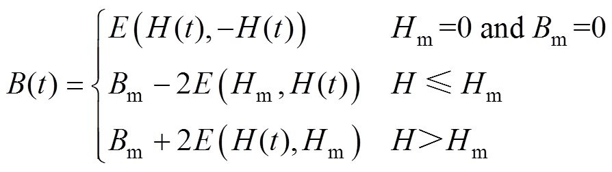 (2)
(2)
式中,Hm、Bm分别为磁滞回线上一回转点对应的磁场强度与磁通密度。式(2)的三个表达式分别用于模拟磁性材料的初始磁化曲线、磁滞回线下降支与上升支。
为得到解析形式的正Preisach模型,课题组首先利用特殊形式的解析函数表征了Preisach分布函数,在此基础上推导并得到了解析的Everett函数,从而基于式(2)得到解析的正Preisach模型[23]为
 (3)
(3)
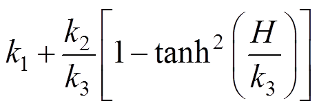
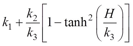
式中,n为Everett函数的项数,ai、bi、gi、k1、k2、k3为模型参数。
需要注意的是,式(3)是课题组针对文献[18](Szabó Z, 2016)存在的推导失误、不通用等问题,而重新推导并提出的目前首个正确且通用的解析正Preisach模型。该模型的具体推导过程和其与文献[18]的区别请读者参阅课题组近期已发表的研究成果——《解析正Preisach磁滞模型的推导与修 正》[23]。
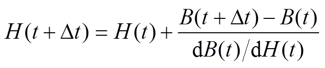
若已知某一时刻t的磁导率dB(t)/dH(t)的解析表达式,则下一时刻t+Dt的磁场强度H(t+Dt)可通过式(4)求得。
 (4)
(4)
式中,B(t+Dt)为t+Dt时刻的磁通密度;t时刻的磁导率dB(t)/dH(t)具体表达式可通过第1节解析的正Preisach模型(3)推导而得。
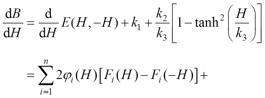
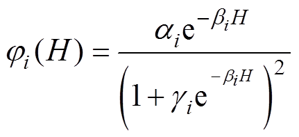
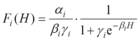
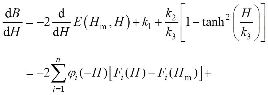
基于解析正Preisach模型的表达式(3),可推导得到初始磁化曲线动态磁导率dB/dH的解析表达式为
 (5)
(5)
其中
 (6)
(6)
 (7)
(7)
同理,可推导磁滞回线下降支与上升支的动态磁导率dB/dH的解析表达式分别为
 (8)
(8)
(9)
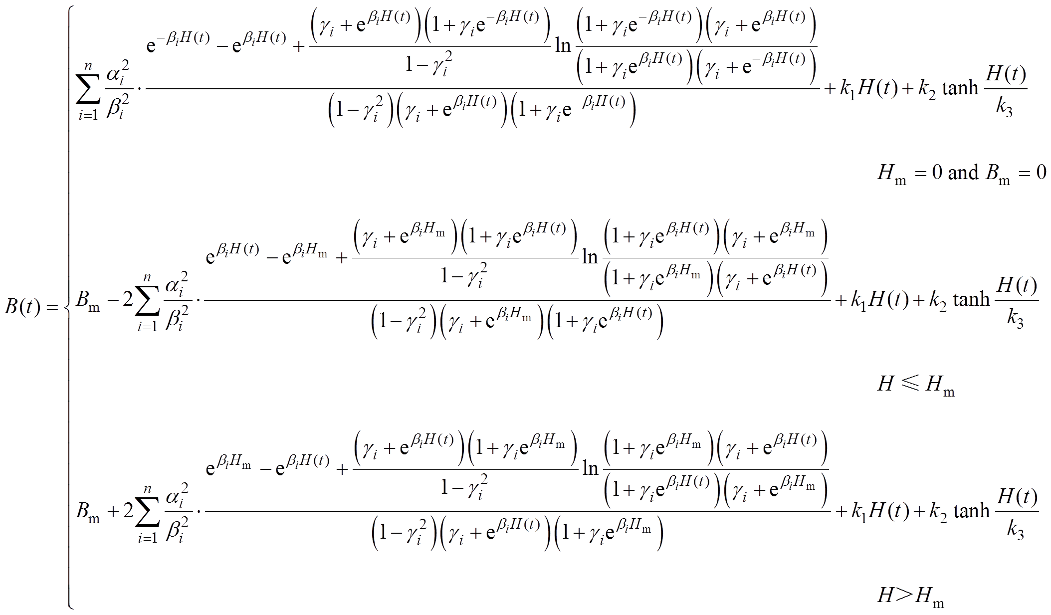
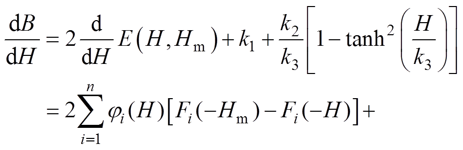
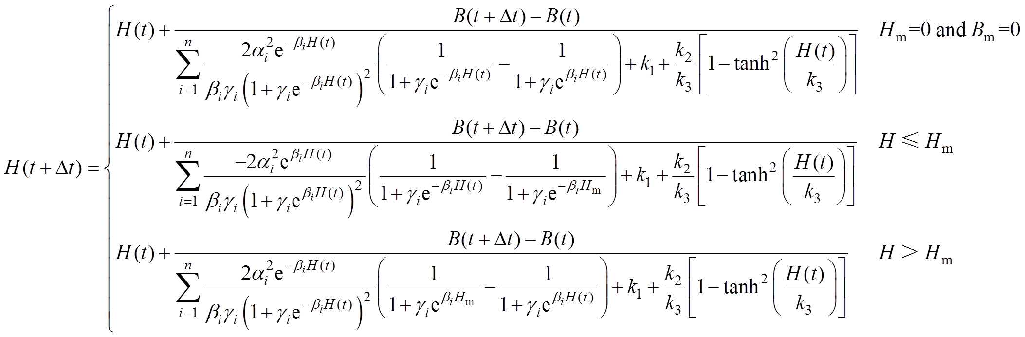
因此,基于本文推导的初始磁化曲线、磁滞回线下降支与上升支的动态磁导率dB/dH的解析表达式(5)、式(8)、式(9),并结合所提磁场强度的差分求解方法(4),即可得到解析逆Preisach模型的数学表达式为
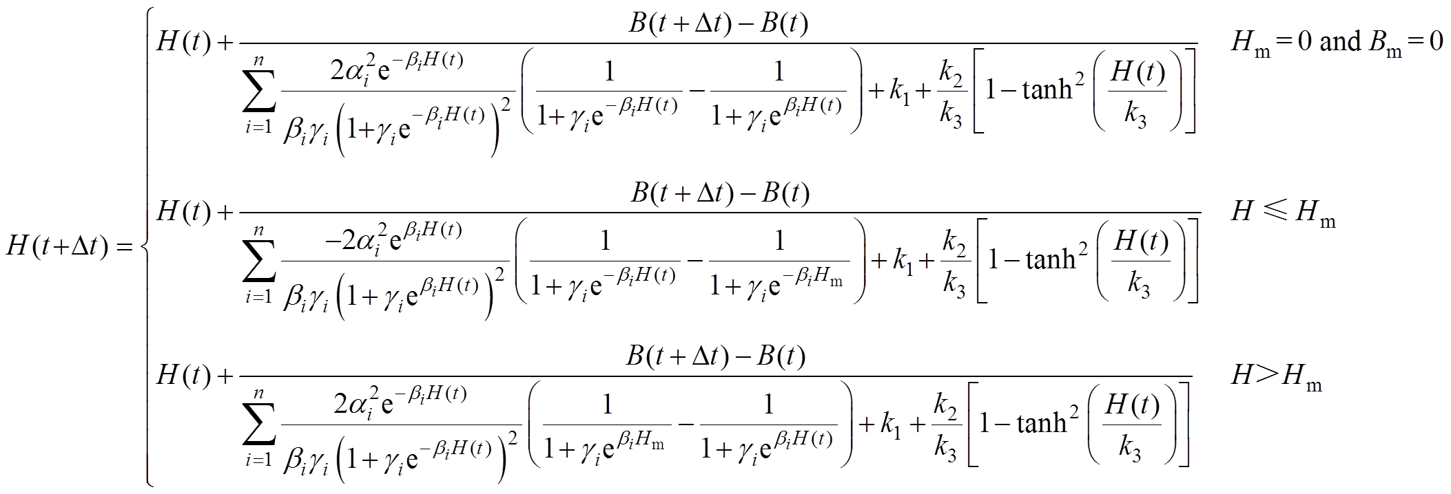 (10)
(10)
基于本文所提解析逆Preisach模型式(10)模拟磁性材料磁滞回线的过程如图1所示。通常,以磁性材料未磁化时的状态(H=0、B=0、Hm=0)作为计算起点。若已知某一时刻的H、Hm,则也可以用此时刻作为计算起点。另外,在计算任意当前t+Dt时刻的磁场强度H(t+Dt)时,上一t时刻的磁场强度H(t)和上一磁化反转点Hm均是已知参数,因而可将式(10)中的H(t)、Hm均看作是已知系数,而输入与输出分别为当前t+Dt时刻的H(t+Dt)、B(t+Dt)。因此,根据逆磁滞模型的定义(当前t+Dt时刻已知的磁通密度、当前t+Dt时刻待求的磁场强度分别作为模型的输入和输出,而与其他已知参数无关),证明了本文所提解析Preisach模型(见式(10))为解析逆Preisach模型。另外也可以从图1所示磁滞回线计算过程不含收敛迭代计算步骤可间接看出所提磁滞模型为逆磁滞模型。
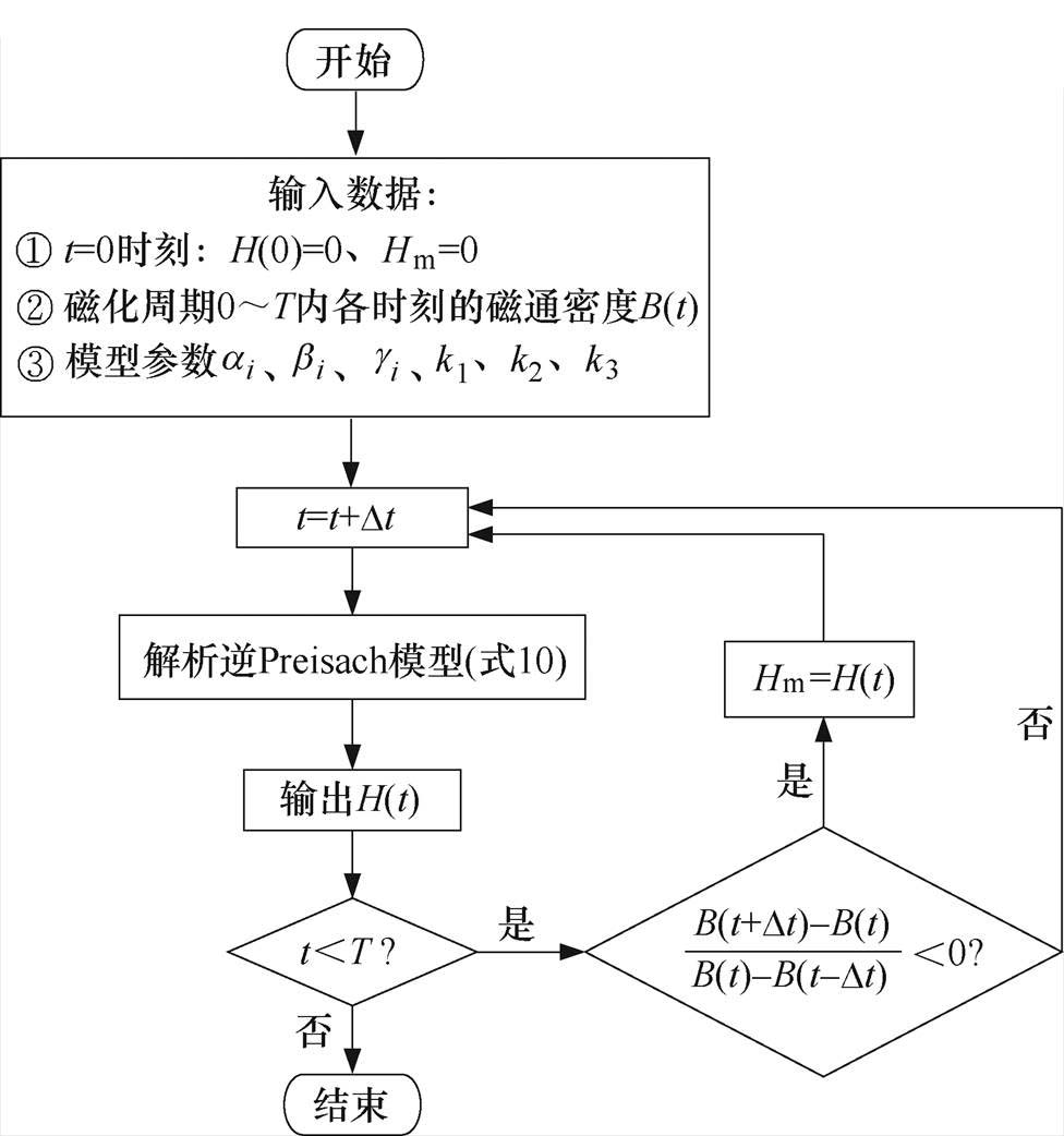
图1 基于所提解析逆Preisach模型模拟磁滞回线的过程
Fig.1 Hysteresis loop simulation process by using the proposed analytical inverse Preisach model
为验证所提解析逆Preisach模型的准确性,本文选用Brockhaus-MPG200磁特性测量系统分别测取了取向硅钢与无取向硅钢两种样品在不同磁通密度下的静态磁滞回线。该测量系统专门用于电工软磁材料的磁特性测量,其测量方法与结果均符合国际电工委员会标准IEC 60404-2[24]。Brockhaus- MPG200磁特性测量系统如图2所示,
根据两种硅钢样品在高、中、低磁通密度下的三条实测磁滞回线(本文选取的取向硅钢样品三条实测磁滞回线的磁通密度峰值分别为1.5 T、1.0 T、0.3 T,而选取的无取向硅钢样品三条实测磁滞回线的磁通密度峰值分别为1.4 T、0.8 T、0.2 T),并利用高效优化算法[24]快速提取的取向及无取向硅钢样品的解析逆Preisach模型参数分别见表1和表2(n=3即可达到较好的模拟效果)。
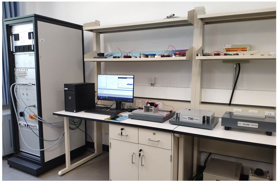
图2 Brockhaus-MPG200磁特性测量系统
Fig.2 Brockhaus-MPG200 magnetic property measuring system
表1 当n=3时,取向硅钢样品的解析逆Preisach模型参数
Tab.1 Parameters of analytical inverse Preisach model of the grain oriented silicon steel sample with n=3
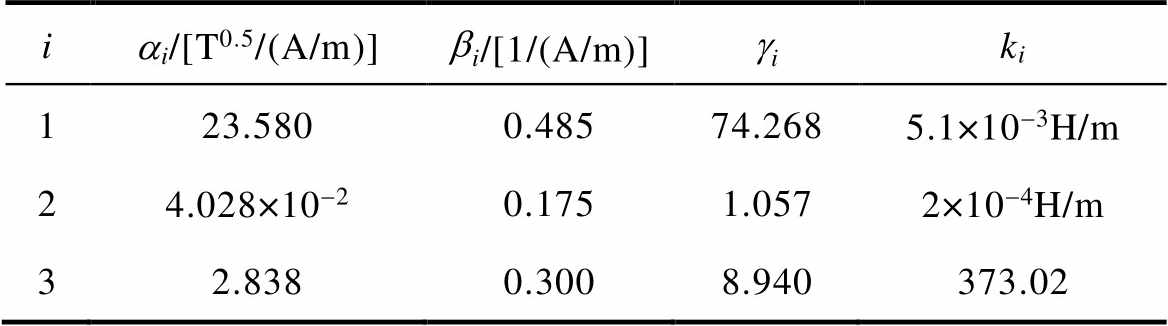
iai/[T0.5/(A/m)]bi/[1/(A/m)]giki 123.5800.48574.2685.1×10-3H/m 24.028×10-20.1751.0572×10-4H/m 32.8380.3008.940373.02
表2 当n=3时,无取向硅钢样品的解析逆Preisach模型参数
Tab.2 Parameters of analytical inverse Preisach model of the non-oriented silicon steel sample with n=3
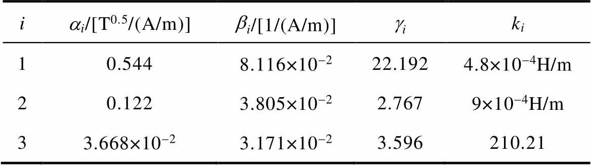
iai/[T0.5/(A/m)]bi/[1/(A/m)]giki 10.5448.116×10-222.1924.8×10-4H/m 20.1223.805×10-22.7679×10⁻⁴H/m 33.668×10-23.171×10-23.596210.21
基于本文所提解析逆Preisach模型模拟的两种硅钢样品在不同磁通密度下的磁滞回线与相应实测磁滞回线的对比结果分别如图3~图6所示。从图3、图5中可以看出,高磁通密度幅值下取向及无取向硅钢样品磁滞回线的模拟结果与相应实测结果在高磁通密度附近区域吻合度稍差,但整体吻合度较好。而从图4、图6可知,在其他磁通密度下基于所提解析逆Preisach模型模拟的磁滞回线与相应实测磁滞回线吻合均较好,从而验证了其在不同磁通密度范围内的模拟精度。
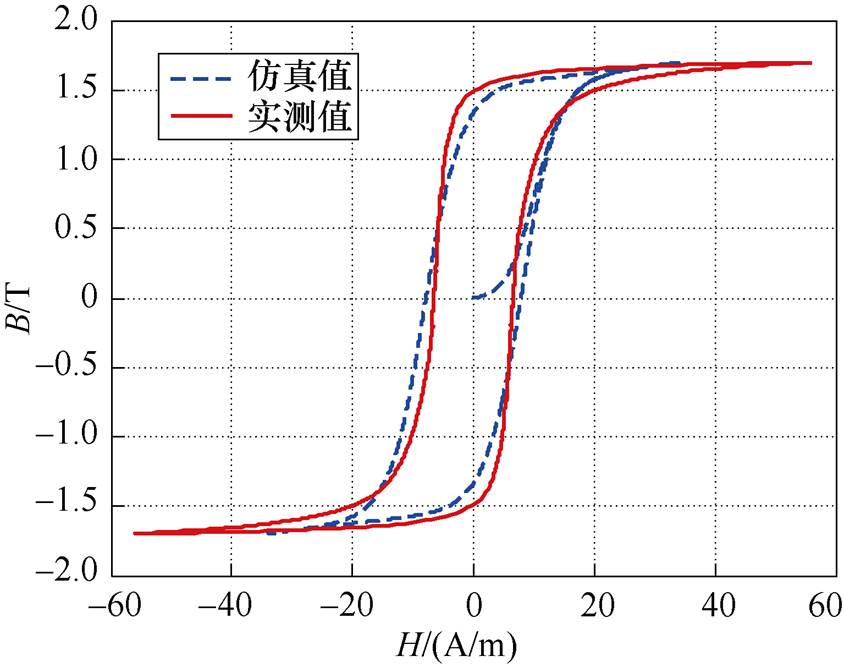
图3 模拟的取向硅钢样品磁滞回线与实测磁滞回线
Fig.3 Simulated and measured hysteresis loops of the grain oriented silicon steel sample
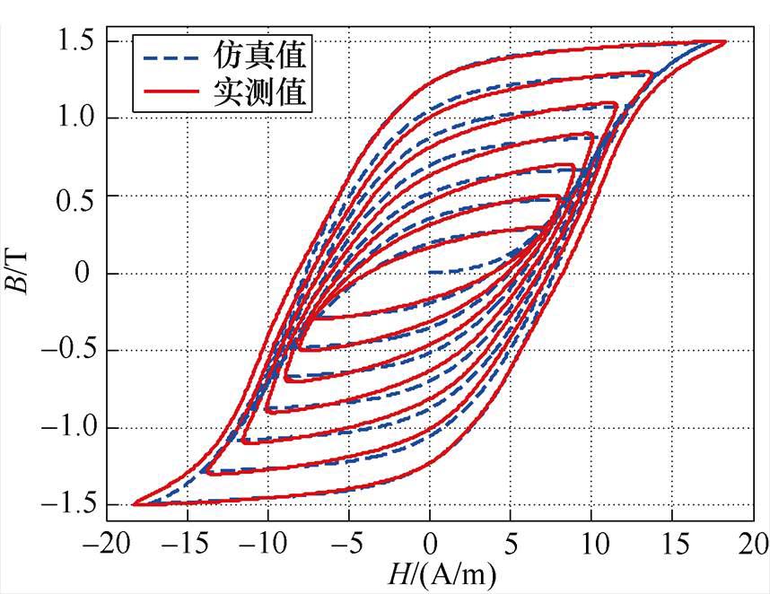
图4 取向硅钢样品在其他不同磁通密度下模拟的磁滞回线与实测磁滞回线
Fig.4 Simulated and measured hysteresis loops of the grain oriented silicon steel sample under other different flux density levels
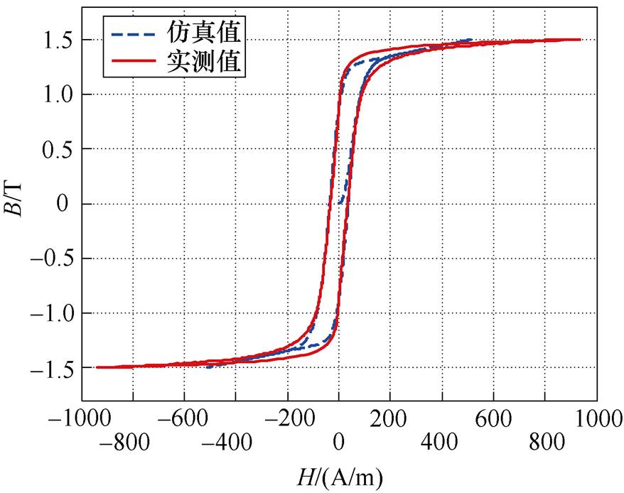
图5 模拟的无取向硅钢样品磁滞回线与实测磁滞回线
Fig.5 Simulated and measured hysteresis loops of the non-oriented silicon steel sample
从当前研究来看,所提解析逆Preisach模型还难以在中低磁通密度磁滞回线具有较高模拟精度的基础上,同时提升高磁通密度磁滞回线的模拟精度。其根本原因在于高磁通密度磁滞回线存在较强的非线性,特别是对于无取向硅钢样品而言(见图5)。需要指出的是,现有逆磁滞模型也均难以实现该目标,这也是为什么目前还有很多学者在研究磁滞模型的根本原因。从图3~图6所示取向及无取向硅钢样品在不同磁通密度下模拟的磁滞回线与实测磁滞回线对比结果可知,所提解析逆Preisach模型已具有较高的全局综合模拟效果。
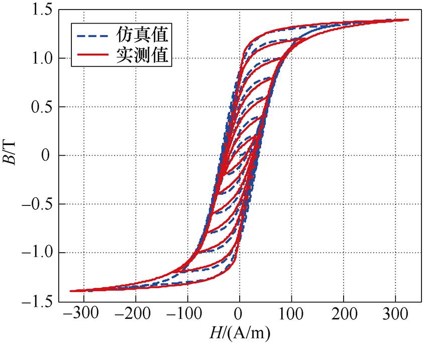
图6 无取向硅钢样品在其他不同磁通密度下模拟的磁滞回线与实测磁滞回线
Fig.6 Simulated and measured hysteresis loops of the non-oriented silicon steel sample under other different flux density levels
另外,所提逆Preisach模型为解析模型,不涉及复杂的参数提取与耗时的迭代求解过程,因而相比于现有不同类型的逆Preisach模型,其计算速度的优势较为明显。
为更加定量地验证所提解析逆Preisach模型的磁滞模拟精度,可将取向与无取向硅钢两类样品在不同磁通密度下的磁滞损耗计算值(等于磁滞回线围成的面积[9])与磁滞损耗测量值进行对比[25],结果分别见表3、表4。另外,引入平均相对误差(Mean Relative Deviation, MRD)的概念,即
 (11)
(11)
式中,m为磁滞回线条数;Wi,cal、Wi,mea分别为第i个磁通密度幅值下模拟的磁滞回线面积与对应的实测磁滞回线面积。对取向及无取向硅钢而言,本文所提解析逆Preisach模型的平均相对误差分别为5.70 %和18.11 %。
此外在模拟精度与求解速度两方面,对比解析逆Preisach模型与目前已被广泛应用的逆J-A模 型[24]。为保证可比性,令两种模型输入磁通密度B的间隔均为0.01 T,也选择取向硅钢样品在磁通密度峰值分别为1.5 T、1.0 T、0.3 T的三条实测磁滞回线,并运用优化算法辨识相应逆J-A模型的参数[24],结果见表5。
表3 基于解析逆Preisach模型计算的取向硅钢样品在不同磁通密度下的磁滞损耗与对应的实测损耗结果对比
Tab.3 Comparison between the calculated losses using analytical inverse Preisach model and the measured losses of the grain oriented silicon steel sample
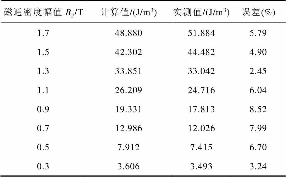
磁通密度幅值Bp/T计算值/(J/m3)实测值/(J/m3)误差(%) 1.748.88051.8845.79 1.542.30244.4824.90 1.333.85133.0422.45 1.126.20924.7166.04 0.919.33117.8138.52 0.712.98612.0267.99 0.57.9127.4156.70 0.33.6063.4933.24
表4 基于解析逆Preisach模型计算的无取向硅钢样品在不同磁通密度下的磁滞损耗与对应的实测损耗结果对比
Tab.4 Comparison between the calculated losses using analytical inverse Preisach model and the measured losses of the non-oriented silicon steel sample
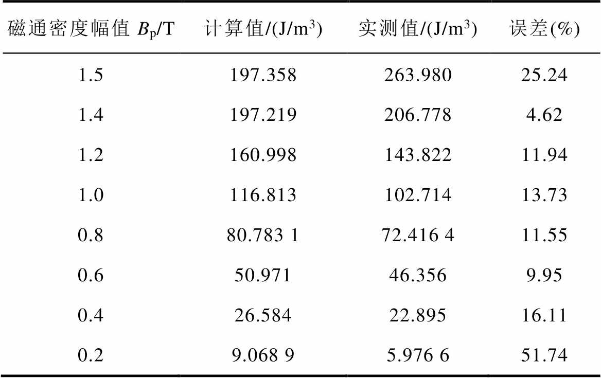
磁通密度幅值Bp/T计算值/(J/m3)实测值/(J/m3)误差(%) 1.5197.358263.98025.24 1.4197.219206.7784.62 1.2160.998143.82211.94 1.0116.813102.71413.73 0.880.783 172.416 411.55 0.650.97146.3569.95 0.426.58422.89516.11 0.29.068 95.976 651.74
表5 取向硅钢样品的逆J-A模型参数
Tab.5 Parameters of inverse J-A model of the grain oriented silicon steel sample
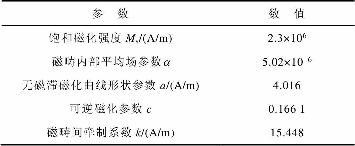
参 数数 值 饱和磁化强度Ms/(A/m)2.3×106 磁畴内部平均场参数a5.02×10-6 无磁滞磁化曲线形状参数a/(A/m)4.016 可逆磁化参数c0.166 1 磁畴间牵制系数k/(A/m)15.448
基于逆J-A模型模拟的取向硅钢样品磁滞回线与相应的实测磁滞回线如图7和图8所示,而基于逆J-A模型计算的磁滞损耗与实测磁滞损耗对比结果见表6。从图7、图8和表6中可以看出,逆J-A模型在高磁通密度与低磁通密度下的磁滞回线模拟精度均较低,其平均相对误差高达16.45 %。
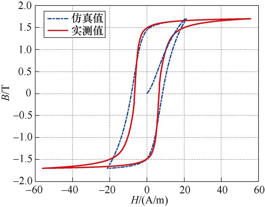
图7 逆J-A模型模拟的取向硅钢样品磁滞回线与实测磁滞回线
Fig.7 Simulated hysteresis loop by inverse J-A model and measured hysteresis loop of the grain oriented silicon steel sample
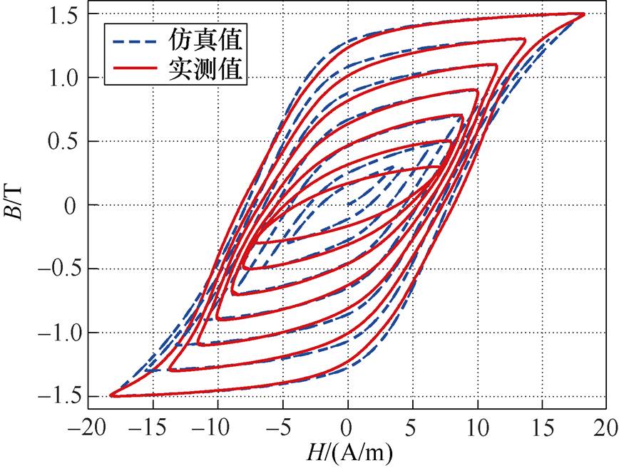
图8 基于逆J-A模型模拟的取向硅钢样品在其他不同磁通密度下的磁滞回线与实测磁滞回线
Fig.8 Simulated hysteresis loops by inverse J-A model and measured hysteresis loops of the grain oriented silicon steel sample under other different flux density levels
为对比本文所提解析逆Preisach模型与逆J-A模型的求解速度,引入时间频度的概念(计算程序中语句执行的次数,通常记为T(n))。本文所提解析逆Preisach模型的时间频度仅约为逆J-A模型的3/8,即说明其求解速度约为逆J-A模型的2.67倍。具体而言,两种模型在模拟磁通密度峰值为1.5T的磁滞回线时,相应的时间频度分别约为2 250、6 000(主要考虑每个时刻计算磁场强度H所需的语句执行次数,其他语句因执行次数较少,通常可忽略)。
表6 基于逆J-A模型计算的取向硅钢样品在不同磁通密度下的磁滞损耗与对应的实测损耗结果对比
Tab.6 Comparison between the calculated losses using inverse J-A model and the measured losses of the grain oriented silicon steel sample
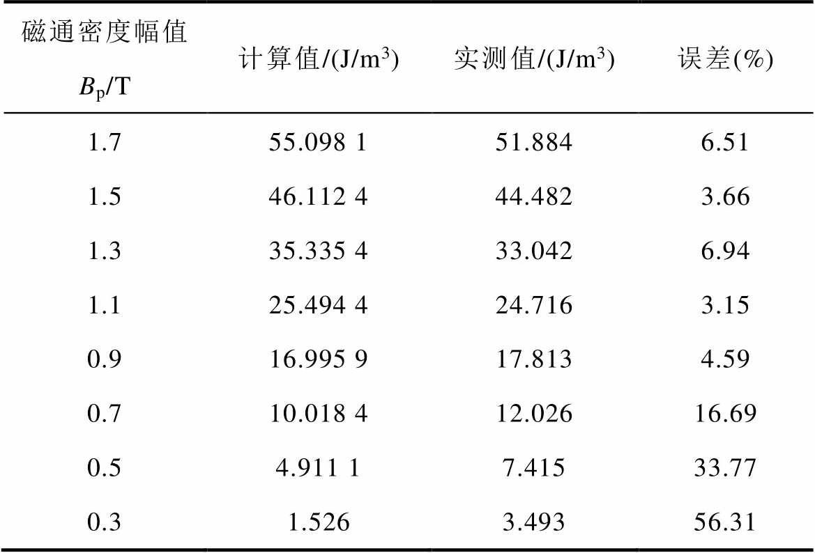
磁通密度幅值Bp/T计算值/(J/m3)实测值/(J/m3)误差(%) 1.755.098 151.8846.51 1.546.112 444.4823.66 1.335.335 433.0426.94 1.125.494 424.7163.15 0.916.995 917.8134.59 0.710.018 412.02616.69 0.54.911 17.41533.77 0.31.5263.49356.31
最后将两种模型的平均相对误差与时间频度汇总,见表7。通过表中对比结果可知,本文所提解析逆Preisach模型在模拟精度与求解速度两方面均明显优于逆J-A模型。
表7 解析逆Preisach模型与逆J-A模型的模拟精度与时间频度对比
Tab.7 Comparison between the time frequencies using analytical inverse Preisach model and inverse J-A model
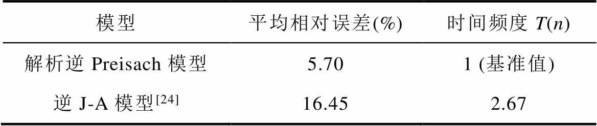
模型平均相对误差(%)时间频度T(n) 解析逆Preisach模型5.701 (基准值) 逆J-A模型[24]16.452.67
逆磁滞模型在软磁材料所属电工装备的电磁热多物理场仿真、电路系统全真模拟、全局结构优化设计等研究领域扮演着重要的角色,一直是国际电磁场领域研究的热点问题。然而,现有不同类型的逆Preisach磁滞模型因不是解析模型而存在参数提取过程复杂繁琐、求解时间长、稳定性差等诸多问题,造成它们在实际工程中的实用性较低。提出模拟精度高的解析逆Preisach模型是解决现有问题的关键所在,但尚未见到相关研究报道。本文在课题组所提首个正确且通用的解析正Preisach模型的基础上,推导并提出了目前唯一一个解析形式的逆Preisach模型。为验证该模型的准确性,测量了取向及无取向硅钢两类不同软磁材料样品在不同磁通密度下的磁滞回线,并将其与模拟的磁滞回线进行了详细对比分析,发现两者吻合情况较好,验证了所提解析逆Preisach模型的精度。另外在模拟精度与计算速度两方面,将所提解析逆Preisach模型与广泛应用的逆J-A模型进行了对比,发现该模型的平均相对误差仅为5.70 %,而逆J-A模型却高达16.45 %,且其计算速度是逆J-A模型的2.67倍。因此,本文所提解析逆Preisach模型相比于逆J-A等磁滞模型具有更为优异的综合性能。
参考文献
[1] 赵小军, 王瑞, 杜振斌, 等. 交直流混合激励下取向硅钢片磁滞及损耗特性模拟方法[J]. 电工技术学报, 2021, 36(13): 2791-2800.
Zhao Xiaojun, Wang Rui, Du Zhenbin, et al. Hysteretic and loss modeling of grain oriented silicon steel lamination under AC-DC hybrid magneti- zation[J]. Transactions of China Electrotechnical Society, 2021, 36(13): 2791-2800.
[2] 赵小军, 曹越芝, 刘兰荣, 等. 交直流混合激励下变压器用叠片式磁构件杂散损耗问题的数值模拟及实验验证[J]. 电工技术学报, 2021, 36(1): 141- 150.
Zhao Xiaojun, Cao Yuezhi, Liu Lanrong, et al. Numerical simulation and experimental verification of stray loss of laminated magnetic components for transformers under AC-DC hybrid excitation[J]. Transactions of China Electrotechnical Society, 2021, 36(1): 141-150.
[3] 赵志刚, 徐曼, 胡鑫剑. 基于改进损耗分离模型的铁磁材料损耗特性研究[J]. 电工技术学报, 2021, 36(13): 2782-2790.
Zhao Zhigang, Xu Man, Hu Xinjian. Research on magnetic losses characteristics of ferromagnetic materials based on improvement loss separation model[J]. Transactions of China Electrotechnical Society, 2021, 36(13): 2782-2790.
[4] 刘任, 李琳. 基于场分离技术与损耗统计理论的动态Energetic磁滞模型[J]. 中国电机工程学报, 2019, 39(增刊): 6412-6418.
Liu Ren, Li Lin. Dynamic energetic hysteresis model based on field separation technology and loss statistics theory[J]. Proceedings of the CSEE, 2019, 39(S): 6412-6418.
[5] Luo Min, Dujic D, Allmeling J. Modeling frequency- dependent core loss of ferrite materials using permeance–capacitance analogy for system-level circuit simulations[J]. IEEE Transactions on Power Electronics, 2019, 34(4): 3658-3676.
[6] Dlala E. Efficient algorithms for the inclusion of the Preisach hysteresis model in nonlinear finite-element methods[J]. IEEE Transactions on Magnetics, 2011, 47(2): 395-408.
[7] de la Barrière O, Ragusa C, Appino C, et al. Prediction of energy losses in soft magnetic materials under arbitrary induction waveforms and DC bias[J]. IEEE Transactions on Industrial Electronics, 2017, 64(3): 2522-2529.
[8] 李伊玲, 李琳, 刘任, 等. 基于非均匀单元离散法的静态逆Preisach模型分布函数辨识[J]. 中国电机工程学报, 2021, 41(15): 5340-5351.
Li Yiling, Li Lin, Liu Ren, et al. The non-uniform element discretization method for identifying dis- tribution function of static inverse Preisach model[J]. Proceedings of the CSEE, 2021, 41(15): 5340-5351.
[9] Liu Ren, Li Lin. Analytical prediction model of energy losses in soft magnetic materials over broadband frequency range[J]. IEEE Transactions on Power Electronics, 2021, 36(2): 2009-2017.
[10] Bi Shasha, Sutor A, Lerch R, et al. An efficient inverted hysteresis model with modified switch operator and differentiable weight function[J]. IEEE Transactions on Magnetics, 2013, 49(7): 3175-3178.
[11] Bi Shasha, Wolf F, Lerch R, et al. An inverted Preisach model with analytical weight function and its numerical discrete formulation[J]. IEEE Transactions on Magnetics, 2014, 50(11): 1-4.
[12] Zirka S E, Moroz Y I, Harrison R G, et al. Inverse hysteresis models for transient simulation[J]. IEEE Transactions on Power Delivery, 2014, 29(2): 552- 559.
[13] Mayergoyz I. Mathematical models of hysteresis[J]. IEEE Transactions on Magnetics, 1986, 22(5): 603- 608.
[14] 刘任, 李琳, 乔光尧, 等. 考虑偏置小磁滞回环的非正弦激励下磁性材料损耗计算方法[J]. 中国电机工程学报, 2020, 40(19): 6093-6103.
Liu Ren, Li Lin, Qiao Guangyao, et al. Calculation method of magnetic material losses under non- sinusoidal excitation considering the biased minor loops[J]. Proceedings of the CSEE, 2020, 40(19): 6093-6103.
[15] 赵小军, 刘小娜, 肖帆, 等. 基于Preisach模型的取向硅钢片直流偏磁磁滞及损耗特性模拟[J]. 电工技术学报, 2020, 35(9): 1849-1857.
Zhao Xiaojun, Liu Xiaona, Xiao Fan, et al. Hysteretic and loss modeling of silicon steel sheet under the DC biased magnetization based on the Preisach model[J]. Transactions of China Electrotechnical Society, 2020, 35(9): 1849-1857.
[16] Li Zhi, Shan Jinjun, Gabbert U. Inverse compensator for a simplified discrete Preisach model using model- order reduction approach[J]. IEEE Transactions on Industrial Electronics, 2019, 66(8): 6170-6178.
[17] Szabó Z. Preisach functions leading to closed form permeability[J]. Physica B: Condensed Matter, 2006, 372(1/2): 61-67.
[18] Szabó Z, Füzi J. Implementation and identification of Preisach type hysteresis models with Everett Function in closed form[J]. Journal of Magnetism and Magnetic Materials, 2016, 406: 251-258.
[19] Fallah E, Badeli V. A new approach for modeling of hysteresis in 2-D time-transient analysis of eddy current using FEM[J]. IEEE Transactions on Mag- netics, 2017, 53(7): 1-14.
[20] Cao Yue, Xu Ke, Jiang Weilin, et al. Hysteresis in single and polycrystalline iron thin films: major and minor loops, first order reversal curves, and Preisach modeling[J]. Journal of Magnetism and Magnetic Materials, 2015, 395: 361-375.
[21] Sadowski N, Batistela N J, Bastos J P A, et al. An inverse Jiles-Atherton model to take into account hysteresis in time-stepping finite-element calcula- tions[J]. IEEE Transactions on Magnetics, 2002, 38(2): 797-800.
[22] Cardelli E, Torre E D, Tellini B. Direct and inverse Preisach modeling of soft materials[J]. IEEE Transa- ctions on Magnetics, 2000, 36(4): 1267-1271.
[23] 刘任, 杜莹雪, 李琳, 等. 解析正Preisach磁滞模型的推导与修正[J]. 中国电机工程学报, 2023, 43(5): 2070-2079.
Liu Ren, Du Yingxue, Li Lin, et al. Derivation and modification of analytical forward Preisach hysteresis model[J]. Proceedings of the CSEE, 2023, 43(5): 2070-2079.
[24] 刘任, 李琳, 王亚琦, 等. 基于随机性与确定性混合优化算法的Jiles-Atherton磁滞模型参数提取[J]. 电工技术学报, 2019, 34(11): 2260-2268.
Liu Ren, Li Lin, Wang Yaqi, et al. Parameter extraction for Jiles-Atherton hysteresis model based on the hybrid technique of stochastic and deter- ministic optimization algorithm[J]. Transactions of China Electrotechnical Society, 2019, 34(11): 2260- 2268.
[25] Liu Ren, Li Lin. Accurate symmetrical minor loops calculation with a modified energetic hysteresis model[J]. IEEE Transactions on Magnetics, 2020, 56(3): 1-4.
Abstract The complex nonlinear hysteresis characteristics of soft magnetic materials significantly impact the energy losses, multi-physics field, and other properties of electrical equipment. Thus, it is crucial to accurately simulate the hysteresis loops of the soft magnetic materials. Under this circumstance, many hysteresis models, such as the well-known Preisach and Jiles-Atherton (J-A) models, have been developed. As the FEA problem of the electrical equipment is usually formulated by magnetic vector potential, making the magnetic flux density B the output of the differential equations, the inverse hysteresis models are more in demand. The inverse Preisach model is usually viewed as the most accurate among all the inverse hysteresis models. However, it involves complex integral operations, so its computation cost is high. As a result, it is not practical in electrical engineering, which makes the accurate analytical inverse Preisach model inheriting low computation cost more desired.
In this paper, to our knowledge, an analytical inverse Preisach model, the only one among all of the Preisach models, is developed and proposed. Firstly, the analytical expressions of permeability of the initial magnetization curve, ascending and descending segments of the hysteresis loop are obtained using our proposed analytical forward Preisach hysteresis model based on the analytical Everett function. The analytical inverse Preisach hysteresis model, as shown in Eq.(1), is derived with the difference method. A grain-oriented silicon steel sample and a non-oriented silicon steel sample are selected to measure their hysteresis loops at different flux density levels. The simulated hysteresis loops and the measured ones are compared. It is shown that the predicted hysteresis loops agree with the measured ones. Additionally, each calculated hysteresis loss (the area enclosed by the corresponding simulated hysteresis loop) is compared with the measured one, which also tests the accuracy of our proposed model. Besides, the average relative error of the analytical inverse Preisach model is smaller than that of the inverse J-A model by more than 10%, and its computation speed is approximately 2.67 times faster than that of the inverse J-A model.
 (A1)
(A1)
where ai, bi, gi, k1 ,k2, k3 are the model coefficients, n is the number of items in Everett function, Hm and Bm are the last reversal magnetic field intensity and magnetic flux density, respectively.
keywords:Soft magnetic materials, hysteresis model, analytical inverse Preisach model
DOI: 10.19595/j.cnki.1000-6753.tces.220467
中图分类号:TM464
湖北省教育厅科学技术研究计划青年人才项目(Q20221205)和宜昌市科技计划项目(A23-4-09)资助。
收稿日期 2022-03-29
改稿日期 2022-08-06
刘 任 男,1990年生,博士,硕士生导师,主要研究方向为电工软磁材料的宽频磁化与损耗机理及其建模方法和电工装备的电磁综合特性分析与全局结构优化设计。E-mail: liu_remail@sina.com(通信作者)
杜莹雪 女,1994年生,硕士,研究方向为电工软磁材料的磁滞及损耗建模方法。E-mail: 18222243479@163.com
(编辑 郭丽军)