图1 四回非全线平行输电线路物理模型
Fig.1 Physical model of quadruple-circuit non-full parallel transmission lines
摘要 随着电力系统的不断发展,输电走廊日益狭窄,四回线路共用一部分走廊的情况非常普遍,目前尚未有相应的线路分布参数测量方法。该文提出一种四回非全线平行线路分布参数精确测量方法,建立四回非全线平行线路的非均匀传输线模型,通过拉普拉斯变换完整地得到四回线路的传输矩阵,获得线路分布参数与线路两端的电压、电流之间关系的数学表达式。在四种独立测量方式下同步测量四回非全线平行线路首末两端的零序电压与零序电流,代入该文所提计算公式,精确求解出24个零序分布参数。通过PSCAD仿真软件证明了该文方法的准确性,并与现有测量方法进行了比较。仿真结果表明,该文方法较现有测量方法具有更高的测量精度。
关键词:四回非全线平行线路 非均匀传输线 零序分布参数 拉普拉斯变换 同步测量
随着电力系统的日益发展,输电网的结构愈加复杂,输电线路的保护显得尤为重要[1]。线路参数的准确测量是输电线路故障测距﹑距离保护﹑短路计算的重要保障[2-6]。由于输电线路所处环境复杂,基于卡松公式的理论计算具有较大的计算误差,因此电力行业规定输电线路参数需要进行实地测量[7-9]。
输电网规模的扩大必然带来输电线路走廊资源的短缺,为解决这一问题,我国广泛采用多回线路平行架设[2, 10-11]。混压四回输电线路已被广泛应用,目前国内外已有500kV/220kV、275kV/132kV等不同电压等级的混压线路[4, 12],未来可能会出现1 000kV/500kV混压线路[13]。混压四回线路通常只有一部分为四回同塔架设,其余部分为双回同塔架设,耦合情况复杂,给参数测量带来了很大的挑战。
多回短距离输电线路集中参数测量方法的研究目前已有较多成果[14-17],这些方法采用集中参数模型,无法测量四回平行线路的分布参数。传统测量方法[14]为单端测量法,步骤繁琐且测量效率低。文献[15]介绍了增量法、干扰法、微分法、相量法等测量输电线路的零序集中参数,总结了这些方法的适用范围。文献[16]采用谐波分量法,利用变压器在饱和状态下产生的3次谐波分量来计算零序电容,可有效地避免工频干扰的影响。文献[17]同步测量线路两端的数据,利用正交距离回归法来估计互感线路的零序集中参数。
目前对于四回线路分布参数测量的研究多数使用四回全线平行架设输电线路模型[18-21]。文献[18]通过测量四组两相系统的开路阻抗和短路阻抗计算零序分布参数。文献[19]结合四回线路末端边界条件,推导出线路分布参数的数学方程组。文献[20]使用拉普拉斯变换法推导了四回线路零序分布参数的数学解析式。然而文献[18-20]对零序分布参数做了过多简化,因而不适用于混压四回线路。对此文献[21]构建了更为准确的线路物理模型,结合传输矩阵测量出混压四回线路的零序分布参数。
目前为止还没有有效的方法可以准确测量四回非全线平行线路的零序分布参数。针对这一现状,本文提出了一种四回非全线平行输电线路零序分布参数的测量方法,考虑到四回线路不同耦合部分电磁环境的差异,将四回耦合部分和双回耦合部分单独处理。配合GPS/北斗的同步授时功能,通过四种独立测量方式,本文测量方法可同时准确求解四回非全线平行输电线路24个零序分布参数。利用PSCAD仿真软件对本文方法和其他方法进行仿真对比。结果表明,本文方法测量精度高,操作步骤少,易于工程应用。
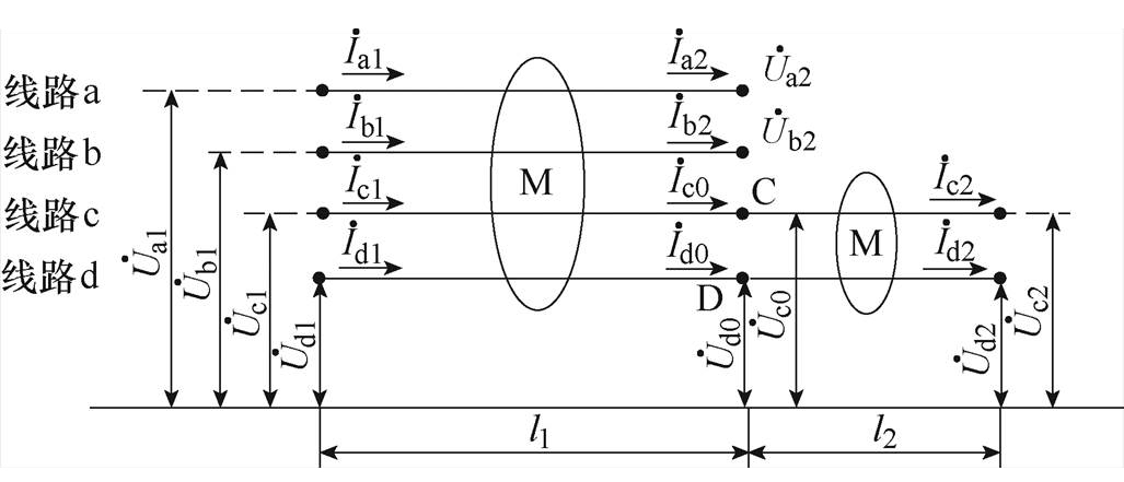
四回非全线平行输电线路有交流四回线路、双回双极直流线路等,且线路架设形式有很多,本文所述的四回非全线平行输电线路分为四回耦合部分和双回耦合部分,其物理模型如图1所示。
图1 四回非全线平行输电线路物理模型
Fig.1 Physical model of quadruple-circuit non-full parallel transmission lines
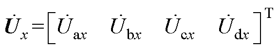
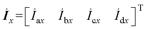
图1中,四回非全线平行输电线路分别用线路a、b、c、d来表示。四回耦合部分的线路长度为l1,双回耦合部分的线路长度为l2,两者的分界点为线路c上的C点与线路d上的D点。由于测量设备安装地点的限制,测量所需的电气量只能从线路的首末端获取。 、
、 、
、 、
、 为各线路首端的电压,
 、
、 、
、 、
、 为各线路首端的电流;
 、
、 、
、 、
、 为各线路末端的电压,
 、
、 、
、 、
、 为各线路末端的电流。
本文所讨论的四回非全线平行线路,由于四回耦合部分与双回耦合部分的电磁耦合情况存在较大的差异,故线路c与线路d为非均匀传输线,下文将四回线路参数分为两部分进行讨论。
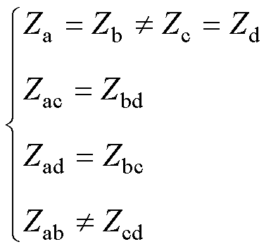
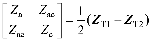
在实际工程中,四回非全线平行线路多数呈现对称分布,某混压四回线路的截面图如图2所示。图2中的四回耦合部分,其零序参数同样也具备一定的对称关系[22],即
 (1)
(1)
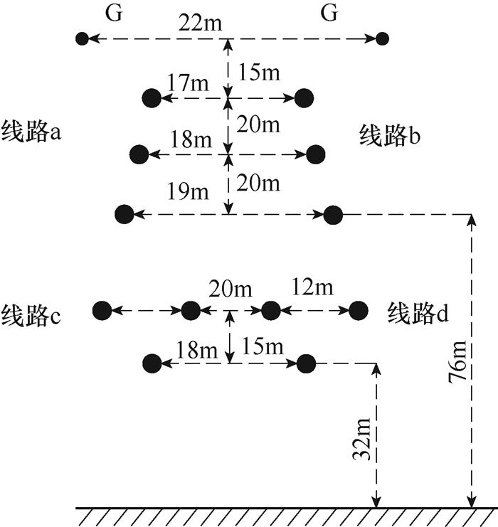
图2 四回耦合部分的截面图
Fig.2 Sectional view of quadruple-circuit coupling part
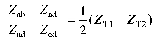
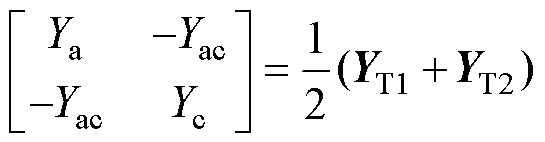
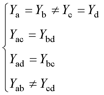 (2)
(2)
式中, 、
、 (
( )分别为四回耦合部分的零序自阻抗和零序自导纳;
 、
、 (
(

 )分别为四回耦合部分两线路间的零序互阻抗和零序互导纳。
线路c与线路d的双回耦合部分也存在对称关系,但这里要注意
 (3)
(3)
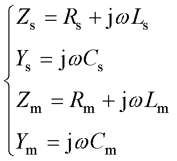
式中, 、
、 分别为双回耦合部分的零序自阻抗和零序自导纳;
 、
、 分别为双回耦合部分的零序互阻抗和零序互导纳。
将上述的零序参数转换为零序电阻、零序电感和零序电容,由于零序电导较小可忽略不计。得
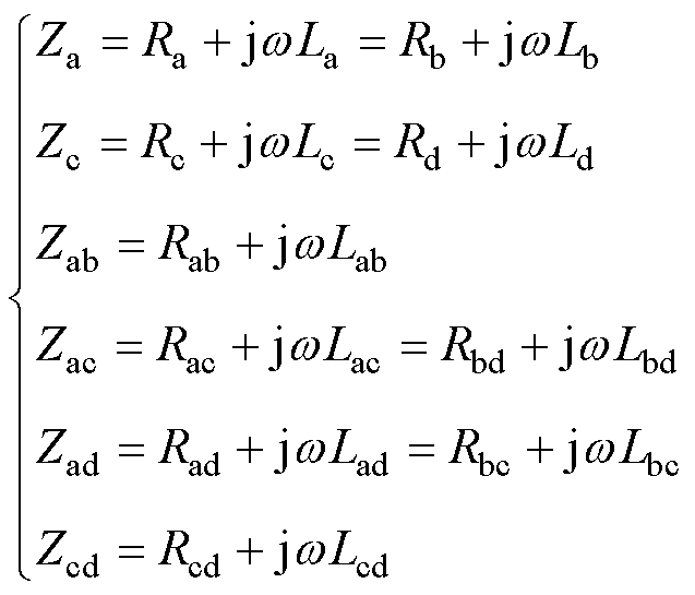 (4)
(4)
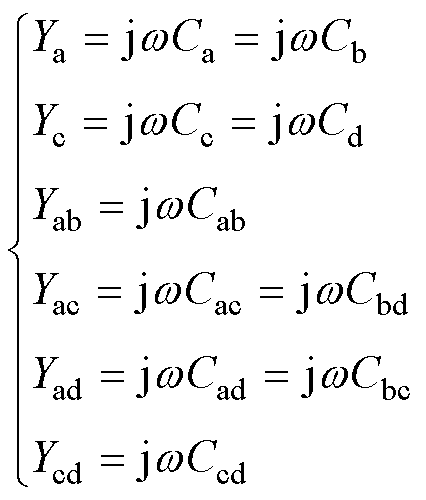 (5)
(5)
式中, 、
、 、
、 分别为四回耦合部分的零序自电阻、零序自电感和零序自电容;
 、
、 、
、 分别为四回耦合部分两线路间的零序互电阻、零序互电感和零序互电容。
 (6)
(6)
式中, 、
、 、
、 分别为双回耦合部分的零序自电阻、零序自电感和零序自电容;
 、
、 、
、 分别为双回耦合部分的零序互电阻、零序互电感和零序互电容。
值得注意的是,互阻抗实部的物理意义为大地电阻。
双回耦合部分的分布参数模型如图3所示。
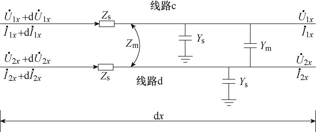
图3 双回耦合部分的分布参数模型
Fig.3 Distributed parameter model of double-circuit coupling part
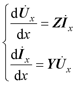
微元 的传输方程如下
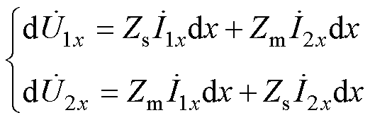 (7)
(7)
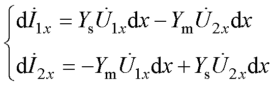 (8)
(8)
对式(7)进行求解,式(8)的求解过程与之相似。设
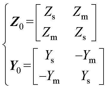 (9)
(9)
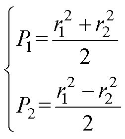
为便于求解,引入乘积矩阵P为
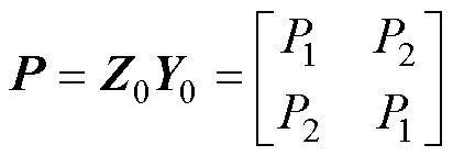 (10)
(10)
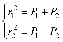
其中
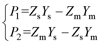
式中,P1、P2为中间变量。
对式(7)进行二阶求导并写成矩阵形式为
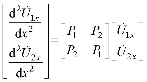 (11)
(11)
对式(11)进行拉普拉斯变换为
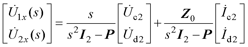 (12)
(12)
式中, 为二阶单位矩阵。
设
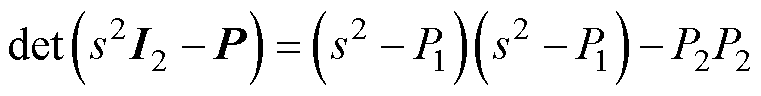
 (13)
(13)
式中, 和
和 为矩阵P的特征根。
由式(13)可得到的关系为
 (14)
(14)
对式(12)进行拉普拉斯逆变换,将 代入得
代入得
 (15)
(15)
式中, 、
、 、
、 、
、 为中间变量参数;
 和
和 分别为图1中C点和D点的零序电压,仅作为中间数学推导使用,并非实测数据。
同理求解式(8)可得
 (16)
(16)
式中, 、
、 为中间变量矩阵参数;
 和
和 分别为C点和D点的零序电流。
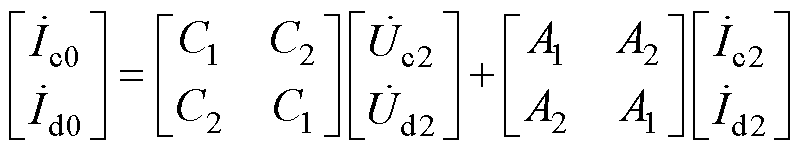
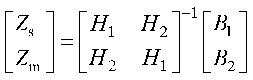
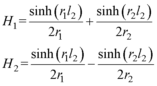
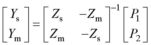
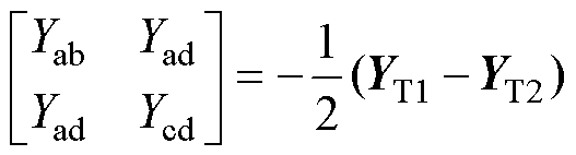
联立式(15)和式(16),得到双回耦合部分的传输矩阵为
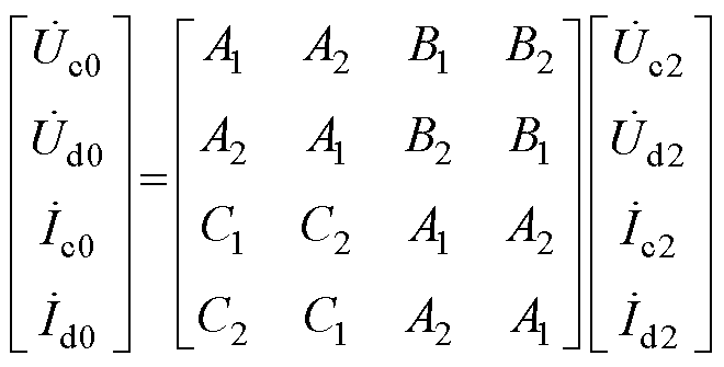 (17)
(17)
式(17)中的中间变量参数表示为
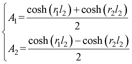 (18)
(18)
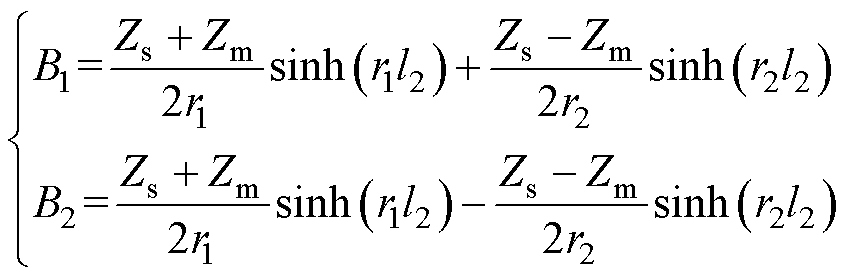 (19)
(19)
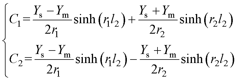 (20)
(20)
四回耦合部分的分布参数模型如图4所示。
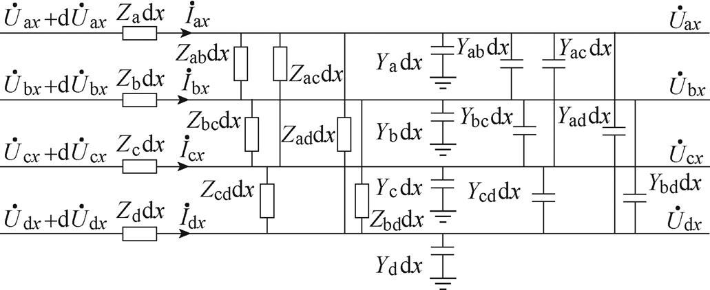
图4 四回耦合部分的分布参数模型
Fig.4 Distributed parameter model of quadruple-circuit coupling part
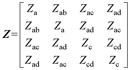
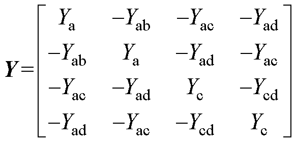
根据基尔霍夫定律列写传输线方程为
 (21)
(21)
其中
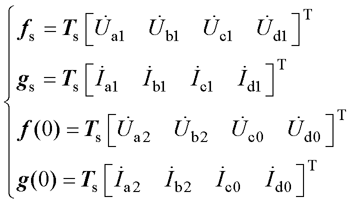
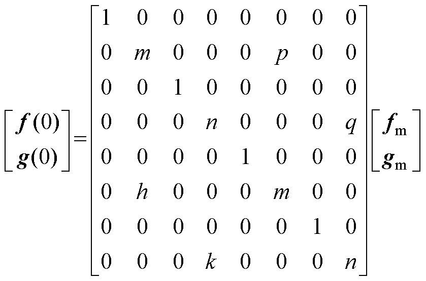
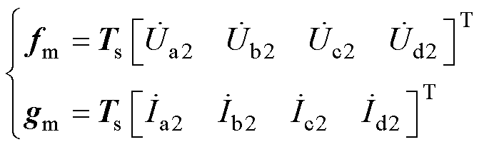
本文引入变换矩阵 ,可以有效地将四维矩阵转化为两个形式高度对称的二维矩阵,降低了求解难度,其表达形式为
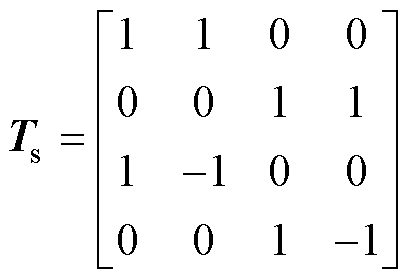 (22)
(22)
代入式(21)可得
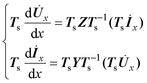 (23)
(23)
设
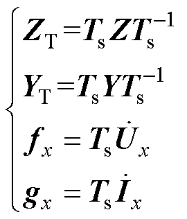 (24)
(24)
则式(23)可改写为
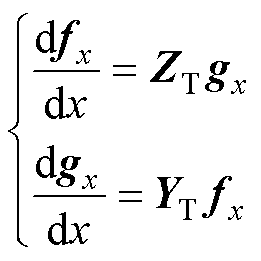 (25)
(25)
其中
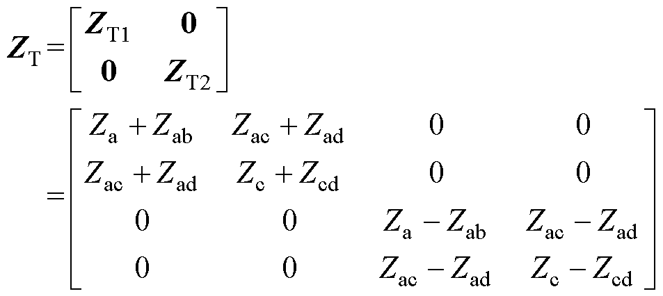
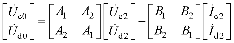
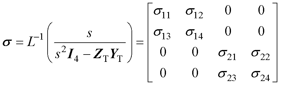
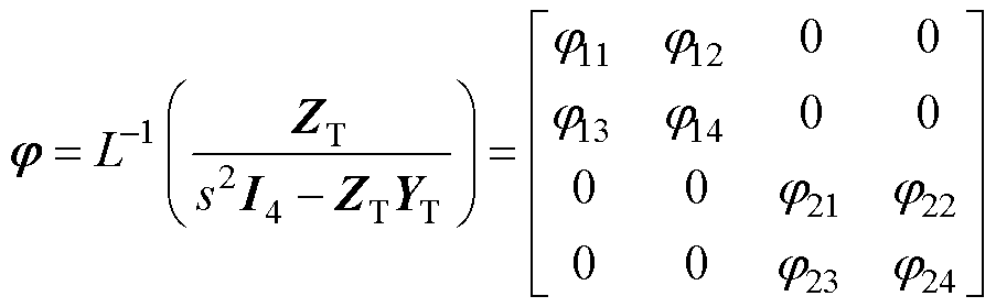
式(25)与式(7)、式(8)形式相同,做同样的拉普拉斯正变换与反变换,并将 代入得到
代入得到
 (26)
(26)
其中
 (27)
(27)
 (28)
(28)
式中, 为取拉普拉斯逆变换。
为便于求解,引入乘积矩阵K,其表达形式为
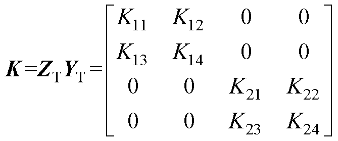 (29)
(29)
中间变量矩阵 和
和 的求解表达式为
 (30)
(30)
 (31)
(31)
其中
 (32)
(32)
式中, 、
、 、
、 、
、 为矩阵K的特征根;
 、
、 、
、 、
、 、
、 、
、 、
、 、
、 为中间变量。
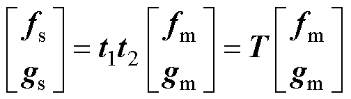
2.1节和2.2节中已求得双回耦合部分与四回耦合部分的传输矩阵,现将式(17)改写成四回线路的传输矩阵形式为
 (33)
(33)
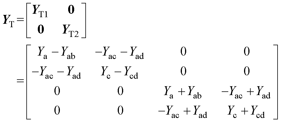
为了使改写后的矩阵能够与四回耦合部分的传输矩阵匹配,对式(33)进行同样的变换,等式两边作T0矩阵的等价变换。T0的表达式为
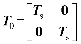 (34)
(34)
式中,0为四阶全零方阵。
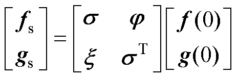
经变换整理得到
 (35)
(35)
其中
令式(26)的传输矩阵为 ,式(35)的传输矩阵为
 ,则联立此二式可得四回非全线平行线路的传输矩阵T,其非零元素具体表达式见附录。
 (36)
(36)
其中
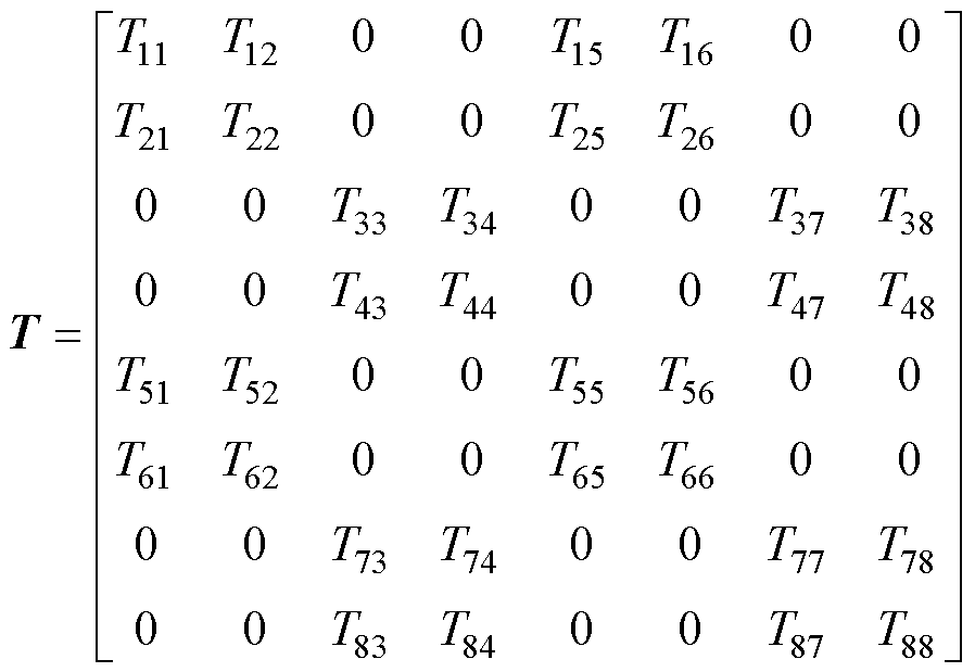
为了测量零序参数,需要获得零序性质的电气量,故需将四回输电线路的首末端分别三相短接,使线路处于零序待测状态。由于四回输电线路的杆塔架构呈对称分布,传输矩阵T有一半的元素为零,使得原本需要八种测量方式,现只需四种测量方式。测量方式的选择有很多种[23],条件是只需满足测量得到的数据代入式(36),便能够解出T中的所有非零元素,表1给出本文的测量方式。需要注意的是,四回线路首端与末端的电气量需要同步测量,利用具有GPS/北斗时间同步功能的测量装置即可实现[24]。
表1 四回输电线路的四种测量方式
Tab.1 Four measurement modes for quadruple-circuit transmission lines
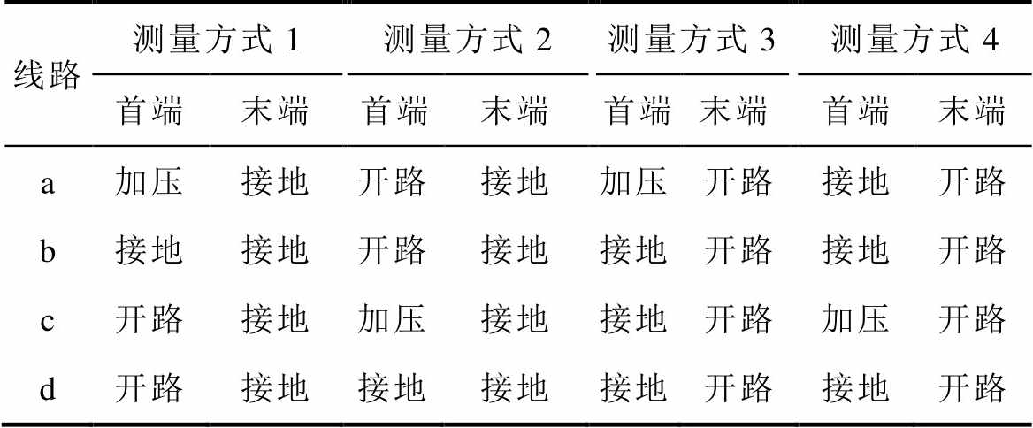
线路测量方式1测量方式2测量方式3测量方式4 首端末端首端末端首端末端首端末端 a加压接地开路接地加压开路接地开路 b接地接地开路接地接地开路接地开路 c开路接地加压接地接地开路加压开路 d开路接地接地接地接地开路接地开路
表1中,“加压”指施加单相工频电源;“接地”指线路三相短接后接地;“开路”指线路三相短接后悬空。需要注意的是,由于对称的缘故,只需四种测量方式,但电源必须施加在线路a和线路c(或者线路b和线路d)上。
1)计算传输矩阵T
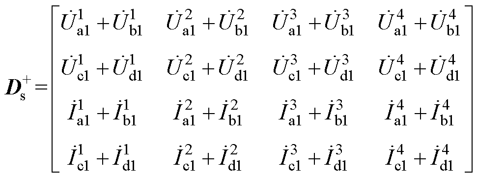
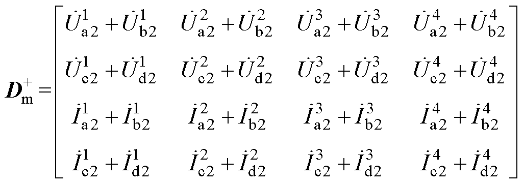
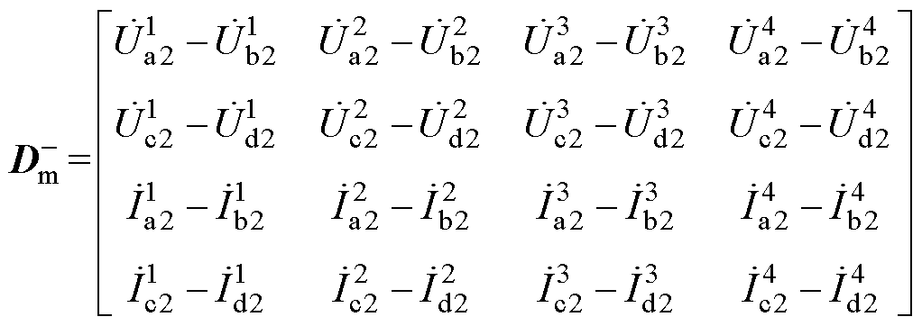
采用表1中的四种测量方式,得到四组四回非全线平行输电线路首末两端的零序电压和零序电流,测量方式采用上标“1~4”来表示,并将这些电气量代入式(36)得到
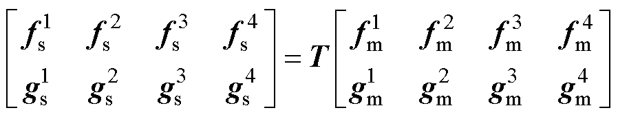 (37)
(37)
将式(37)具体展开得到
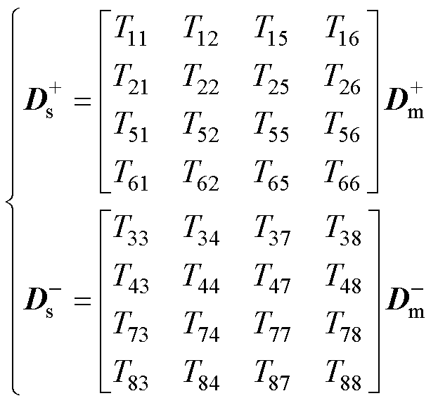 (38)
(38)
其中

由此解得传输矩阵T中的所有非零元素。
2)计算双回耦合部分的中间变量
由式(36)可知
 (39)
(39)
观察矩阵中相同元素( 、
、 、
、 、
、 )所处的位置,可以从矩阵
 中得到计算所需要的等式为
 (40)
(40)
 (41)
(41)
联立式(10)、式(14)、式(18)~式(20)可以得到一个恒等式为
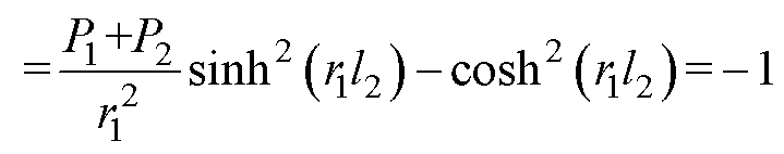 (42)
(42)
同理得到
 (43)
(43)
联立式(40)、式(42)可以得到关于 的一元二次方程为
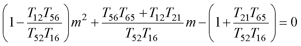 (44)
(44)
解出实部为正的,进而求解 、
、 ;同理联立式(41)、式(43)解得
 、
、 、
、 。
。
3)计算双回耦合部分的零序参数
首先根据式(18)计算特征根 和
和 为
为
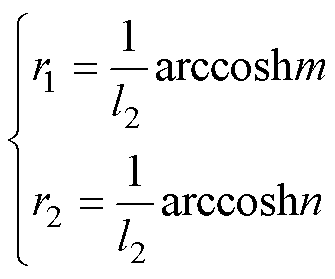 (45)
(45)
再由式(14)计算出P1、P2为
 (46)
(46)
对式(19)进行变换得到
 (47)
(47)
其中
最后根据式(10)得到
 (48)
(48)
将计算得到的 、
、 、
、 、
、 代入式(6)中,转换成双回耦合部分的零序参数。
4)计算四回耦合部分的中间变量
根据附录中 元素的表达式计算中间变量矩阵和的非零元素为
 (49)
(49)
5)计算四回耦合部分的零序参数。首先根据式(30)计算特征根、、、为
 (50)
(50)
根据式(32)计算出中间变量、、、、、、、。
再根据式(30),经过整理可得乘积矩阵K的表达式为
 (51)
(51)
 (52)
(52)
将矩阵,矩阵K,特征根、、、,中间变量、、、代入式(31),可以解得
矩阵 。根据式(29),
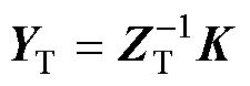 计算可得
计算可得 。最后计算四回耦合部分零序阻抗和零序电纳为
 (53)
(53)
 (54)
(54)
 (55)
(55)
 (56)
(56)
将计算得到的零序阻抗和零序电纳代入式(4)和式(5)中,转换成四回耦合部分的零序参数。
本文根据图2所示的1 000kV/500kV线路结构,利用PSCAD/EMTDC软件搭建仿真模型,如图5所示。仿真采样频率设置为4 000Hz,采样时间设定为1s,选择0.6~0.8s时的仿真数据进行计算。
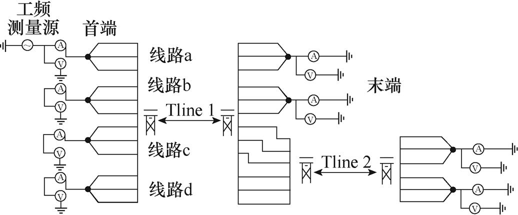
图5 四回非全线平行输电线路仿真模型
Fig.5 Simulation model of quadruple -circuit non-full parallel transmission lines
定义相对测量误差为
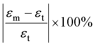 (57)
(57)
式中, 为测量值;
为测量值; 为理论值。
为理论值。
根据PSCAD自动生成的线路信息,可以得到输电线路四回耦合部分与双回耦合部分单位长度零序分布参数的理论值,见表2。
表2 四回非全线平行零序分布参数理论值
Tab.2 Theoretical values of zero sequence parameters of quadruple-circuit non-full parallel transmission lines
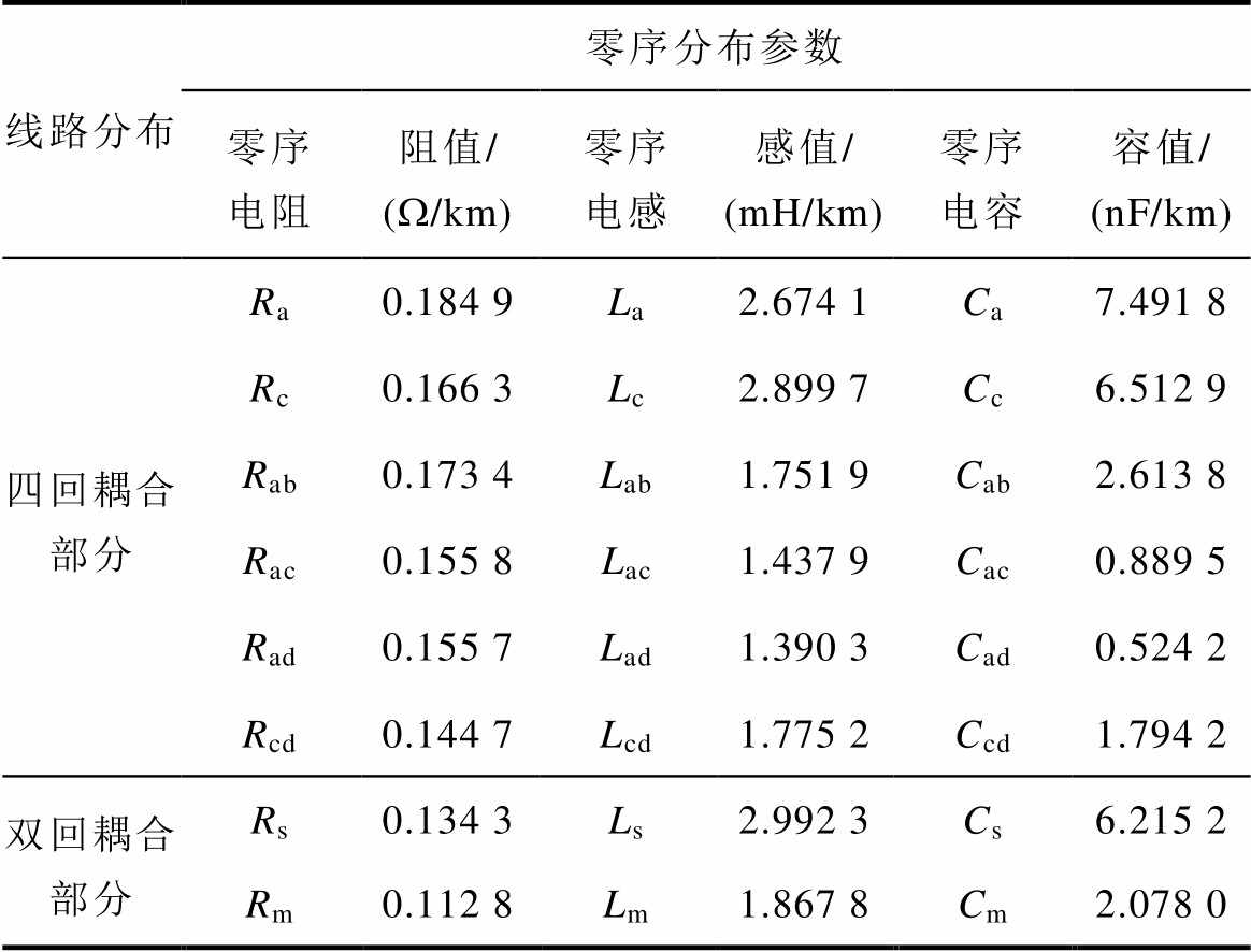
线路分布零序分布参数 零序电阻阻值/ (W/km)零序电感感值/ (mH/km)零序电容容值/ (nF/km) 四回耦合部分Ra0.184 9La2.674 1Ca7.491 8 Rc0.166 3Lc2.899 7Cc6.512 9 Rab0.173 4Lab1.751 9Cab2.613 8 Rac0.155 8Lac1.437 9Cac0.889 5 Rad0.155 7Lad1.390 3Cad0.524 2 Rcd0.144 7Lcd1.775 2Ccd1.794 2 双回耦合部分Rs0.134 3Ls2.992 3Cs6.215 2 Rm0.112 8Lm1.867 8Cm2.078 0
仿真设定双回耦合部分长度l2不变,改变四回耦合部分长度l1,本文方法的仿真测量结果见表3~表5。
表3 本文方法的零序电阻测量结果
Tab.3 Zero sequence resistance measurement results of the proposed method
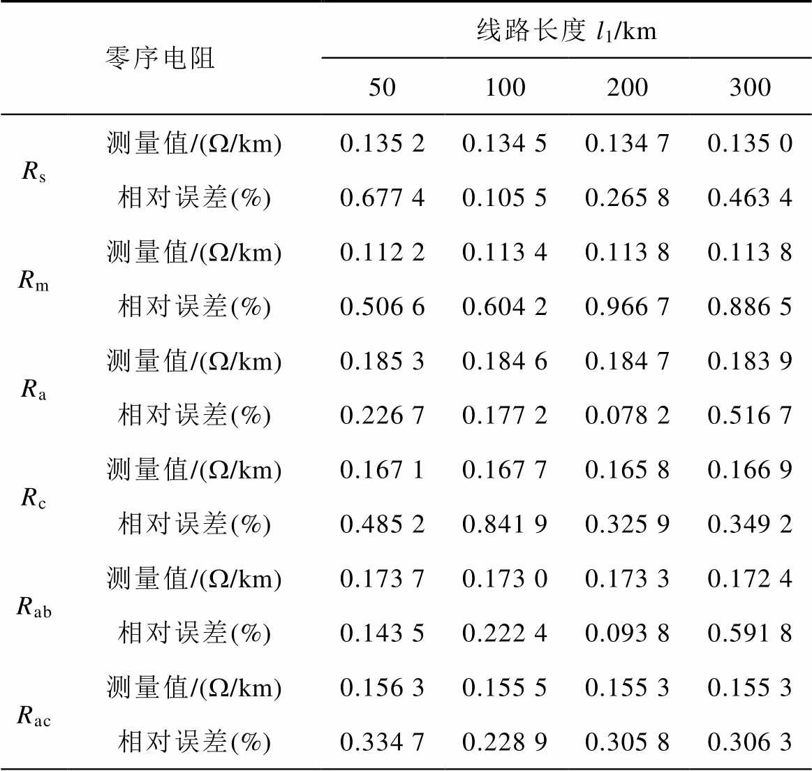
零序电阻线路长度l1/km 50100200300 Rs测量值/(W/km)0.135 20.134 50.134 70.135 0 相对误差(%)0.677 40.105 50.265 80.463 4 Rm测量值/(W/km)0.112 20.113 40.113 80.113 8 相对误差(%)0.506 60.604 20.966 70.886 5 Ra测量值/(W/km)0.185 30.184 60.184 70.183 9 相对误差(%)0.226 70.177 20.078 20.516 7 Rc测量值/(W/km)0.167 10.167 70.165 80.166 9 相对误差(%)0.485 20.841 90.325 90.349 2 Rab测量值/(W/km)0.173 70.173 00.173 30.172 4 相对误差(%)0.143 50.222 40.093 80.591 8 Rac测量值/(W/km)0.156 30.155 50.155 30.155 3 相对误差(%)0.334 70.228 90.305 80.306 3
(续)
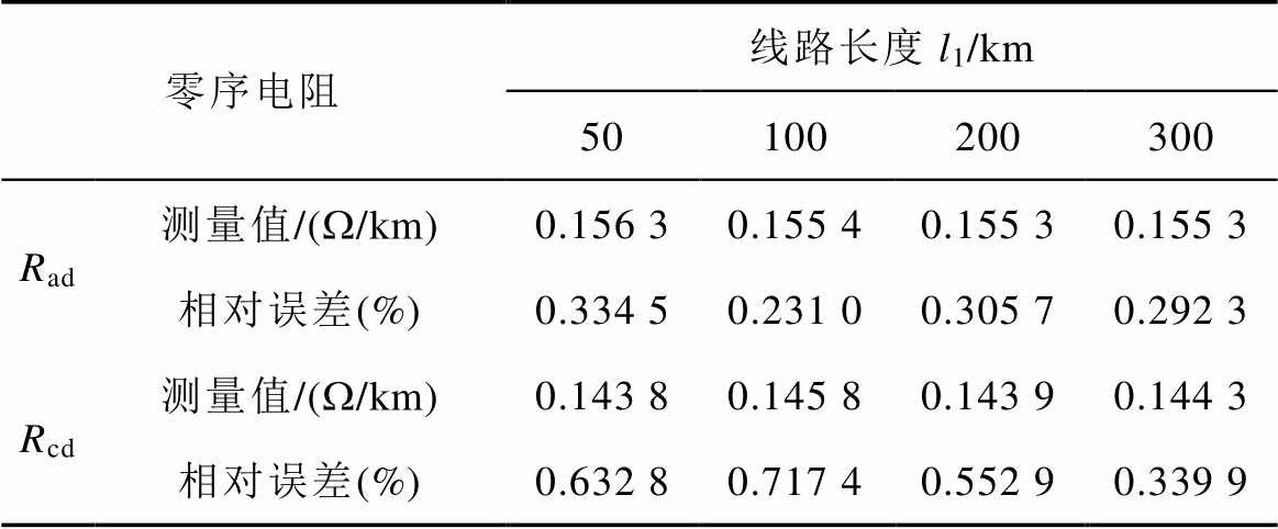
零序电阻线路长度l1/km 50100200300 Rad测量值/(W/km)0.156 30.155 40.155 30.155 3 相对误差(%)0.334 50.231 00.305 70.292 3 Rcd测量值/(W/km)0.143 80.145 80.143 90.144 3 相对误差(%)0.632 80.717 40.552 90.339 9
表4 本文方法的零序电感测量结果
Tab.4 Zero sequence inductance measurement results of the proposed method
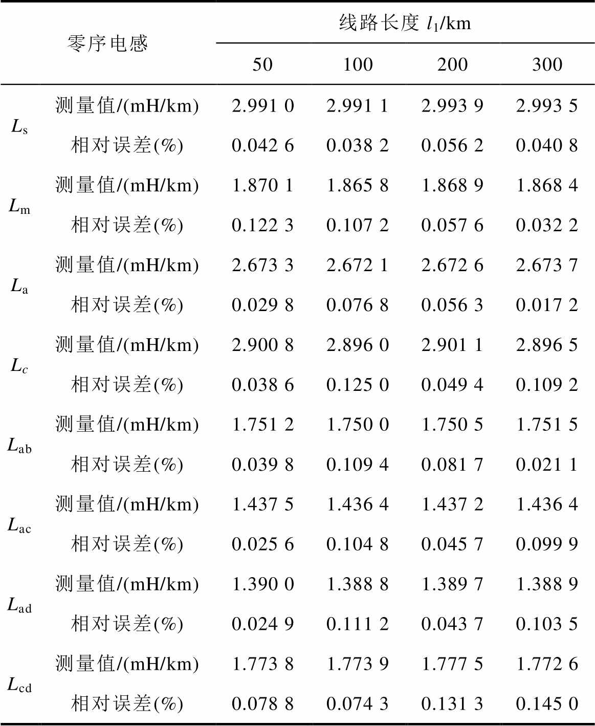
零序电感线路长度l1/km 50100200300 Ls测量值/(mH/km)2.991 02.991 12.993 92.993 5 相对误差(%)0.042 60.038 20.056 20.040 8 Lm测量值/(mH/km)1.870 11.865 81.868 91.868 4 相对误差(%)0.122 30.107 20.057 60.032 2 La测量值/(mH/km)2.673 32.672 12.672 62.673 7 相对误差(%)0.029 80.076 80.056 30.017 2 Lc测量值/(mH/km)2.900 82.896 02.901 12.896 5 相对误差(%)0.038 60.125 00.049 40.109 2 Lab测量值/(mH/km)1.751 21.750 01.750 51.751 5 相对误差(%)0.039 80.109 40.081 70.021 1 Lac测量值/(mH/km)1.437 51.436 41.437 21.436 4 相对误差(%)0.025 60.104 80.045 70.099 9 Lad测量值/(mH/km)1.390 01.388 81.389 71.388 9 相对误差(%)0.024 90.111 20.043 70.103 5 Lcd测量值/(mH/km)1.773 81.773 91.777 51.772 6 相对误差(%)0.078 80.074 30.131 30.145 0
表5 本文方法的零序电容测量结果
Tab.5 Zero sequence capacitance measurement results of the proposed method
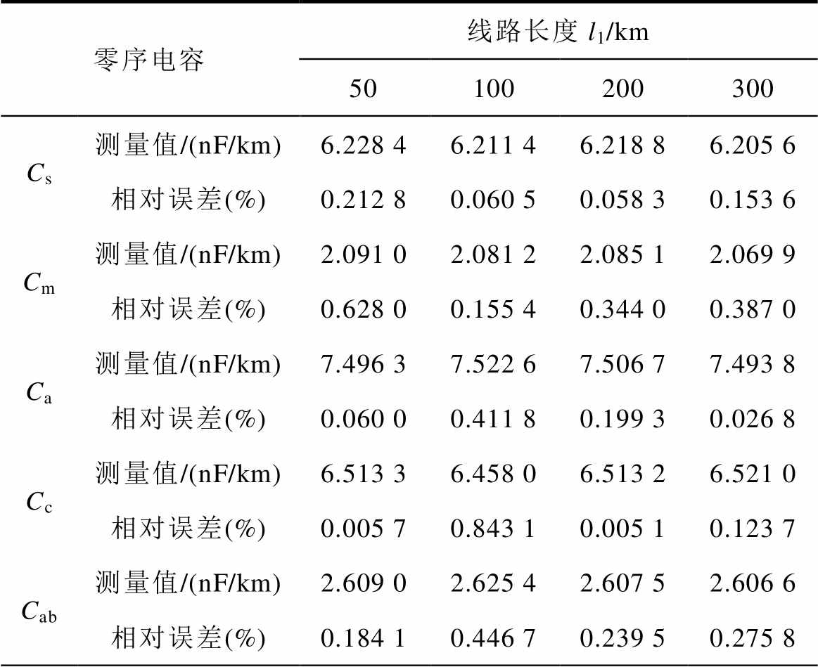
零序电容线路长度l1/km 50100200300 Cs测量值/(nF/km)6.228 46.211 46.218 86.205 6 相对误差(%)0.212 80.060 50.058 30.153 6 Cm测量值/(nF/km)2.091 02.081 22.085 12.069 9 相对误差(%)0.628 00.155 40.344 00.387 0 Ca测量值/(nF/km)7.496 37.522 67.506 77.493 8 相对误差(%)0.060 00.411 80.199 30.026 8 Cc测量值/(nF/km)6.513 36.458 06.513 26.521 0 相对误差(%)0.005 70.843 10.005 10.123 7 Cab测量值/(nF/km)2.609 02.625 42.607 52.606 6 相对误差(%)0.184 10.446 70.239 50.275 8
(续)
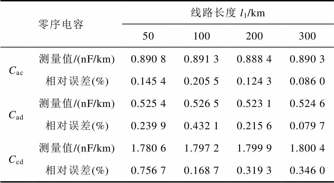
零序电容线路长度l1/km 50100200300 Cac测量值/(nF/km)0.890 80.891 30.888 40.890 3 相对误差(%)0.145 40.205 50.124 30.086 0 Cad测量值/(nF/km)0.525 40.526 50.523 10.524 6 相对误差(%)0.239 90.432 10.215 60.079 7 Ccd测量值/(nF/km)1.780 61.797 21.799 91.800 4 相对误差(%)0.756 70.168 70.319 30.346 0
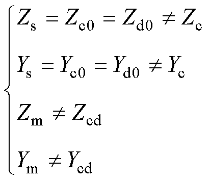
传统方法[14]是一种基于集中参数模型的单端测量法,且在每种测量方式下只能测得一种零序阻抗或零序电纳,因此传统方法在本文模型下需要12种测量方式。需要注意的是,传统方法采用的是均匀传输线模型,即 、
、 、
、 、
、 ,其仿真测量结果见表6。
表6 传统方法的仿真测量结果
Tab.6 Simulation measurement results of the traditional method
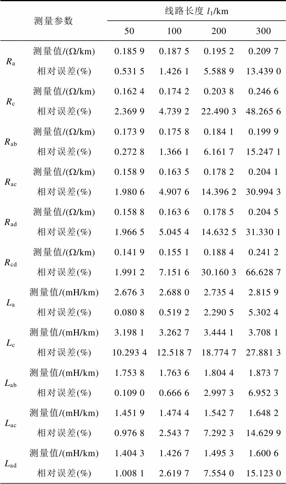
测量参数线路长度l1/km 50100200300 Ra测量值/(W/km)0.185 90.187 50.195 20.209 7 相对误差(%)0.531 51.426 15.588 913.439 0 Rc测量值/(W/km)0.162 40.174 20.203 80.246 6 相对误差(%)2.369 94.739 222.490 348.265 6 Rab测量值/(W/km)0.173 90.175 80.184 10.199 9 相对误差(%)0.272 81.366 16.161 715.247 1 Rac测量值/(W/km)0.158 90.163 50.178 20.204 1 相对误差(%)1.980 64.907 614.396 230.994 3 Rad测量值/(W/km)0.158 80.163 60.178 50.204 5 相对误差(%)1.966 55.045 414.632 531.330 1 Rcd测量值/(W/km)0.141 90.155 10.188 40.241 2 相对误差(%)1.991 27.151 630.160 366.628 7 La测量值/(mH/km)2.676 32.688 02.735 42.815 9 相对误差(%)0.080 80.519 22.290 55.302 4 Lc测量值/(mH/km)3.198 13.262 73.444 13.708 1 相对误差(%)10.293 412.518 718.774 727.881 3 Lab测量值/(mH/km)1.753 81.763 61.804 41.873 7 相对误差(%)0.109 00.666 62.997 36.952 3 Lac测量值/(mH/km)1.451 91.474 41.542 71.648 2 相对误差(%)0.976 82.543 77.292 314.629 9 Lad测量值/(mH/km)1.404 31.426 71.495 31.600 6 相对误差(%)1.008 12.619 77.554 015.123 0
(续)
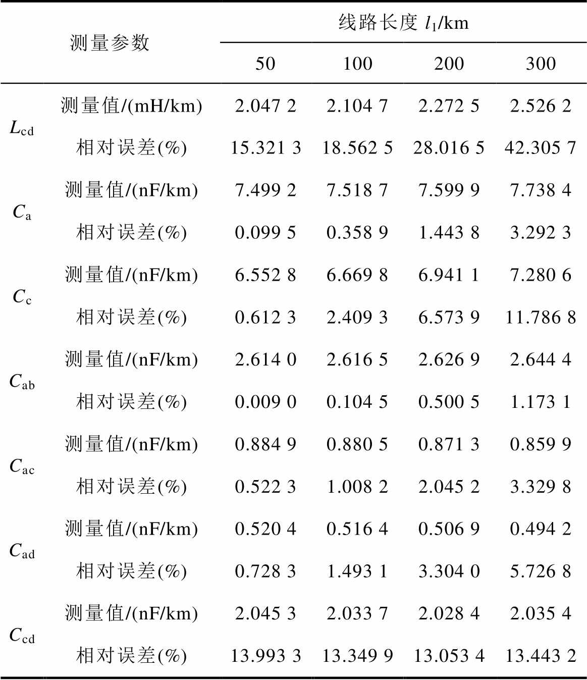
测量参数线路长度l1/km 50100200300 Lcd测量值/(mH/km)2.047 22.104 72.272 52.526 2 相对误差(%)15.321 318.562 528.016 542.305 7 Ca测量值/(nF/km)7.499 27.518 77.599 97.738 4 相对误差(%)0.099 50.358 91.443 83.292 3 Cc测量值/(nF/km)6.552 86.669 86.941 17.280 6 相对误差(%)0.612 32.409 36.573 911.786 8 Cab测量值/(nF/km)2.614 02.616 52.626 92.644 4 相对误差(%)0.009 00.104 50.500 51.173 1 Cac测量值/(nF/km)0.884 90.880 50.871 30.859 9 相对误差(%)0.522 31.008 22.045 23.329 8 Cad测量值/(nF/km)0.520 40.516 40.506 90.494 2 相对误差(%)0.728 31.493 13.304 05.726 8 Ccd测量值/(nF/km)2.045 32.033 72.028 42.035 4 相对误差(%)13.993 313.349 913.053 413.443 2
图6给出本文方法和传统方法在线路长度l1为50~300km时的测量误差对比,图中R、L、C分别为各自相对误差取最大值时四回非全线平行线路的零序电阻、零序电感、零序电容。
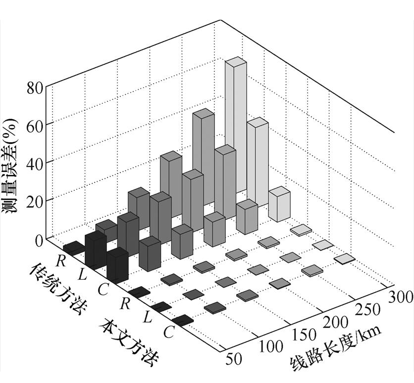
图6 本文方法与传统方法的测量误差对比
Fig.6 Comparison of measurement errors between the proposed method and the traditional method
目前还没有精确的方法计算四回非全线平行线路的零序分布参数,文献[21]给出的方法仅适用于四回全线平行线路,若运用于本文模型,则只能测量 、
、 、
、 、
、 、
、 、
、 。表7为文献[21]方法的仿真测量结果。以零序电容为例,本文方法与文献[21]方法的测量误差对比如图7所示。
分析表3~表7及图6、图7可以得到以下结论:
表7 现有方法的仿真测量结果
Tab.7 Simulation measurement results of the existing method
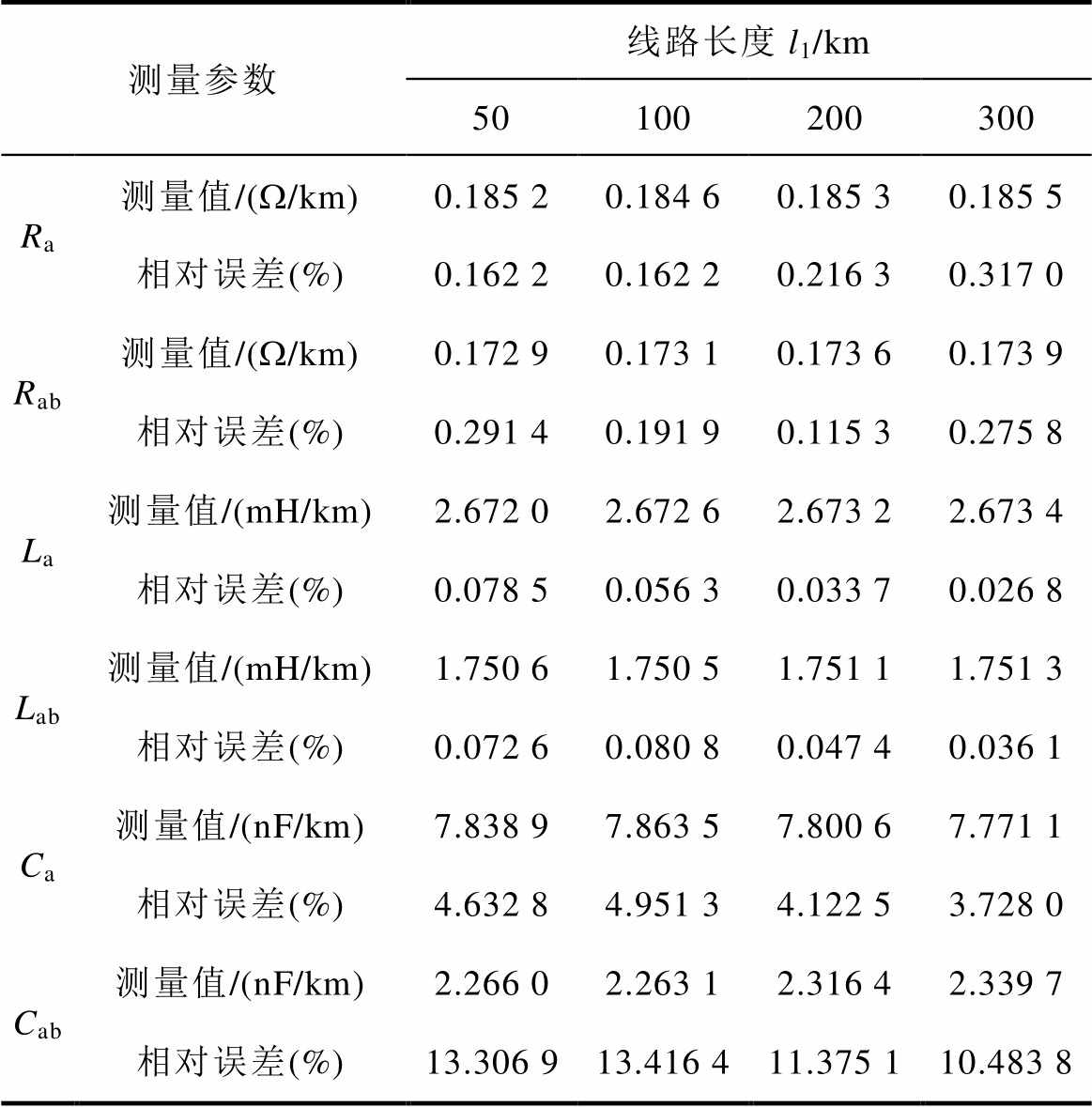
测量参数线路长度l1/km 50100200300 Ra测量值/(W/km)0.185 20.184 60.185 30.185 5 相对误差(%)0.162 20.162 20.216 30.317 0 Rab测量值/(W/km)0.172 90.173 10.173 60.173 9 相对误差(%)0.291 40.191 90.115 30.275 8 La测量值/(mH/km)2.672 02.672 62.673 22.673 4 相对误差(%)0.078 50.056 30.033 70.026 8 Lab测量值/(mH/km)1.750 61.750 51.751 11.751 3 相对误差(%)0.072 60.080 80.047 40.036 1 Ca测量值/(nF/km)7.838 97.863 57.800 67.771 1 相对误差(%)4.632 84.951 34.122 53.728 0 Cab测量值/(nF/km)2.266 02.263 12.316 42.339 7 相对误差(%)13.306 913.416 411.375 110.483 8
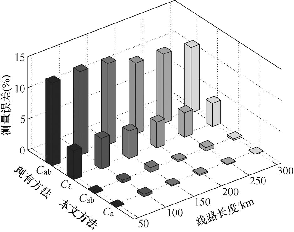
图7 本文方法与现有方法的测量误差对比
Fig.7 Comparison of measurement errors between the proposed method and the existing method
(1)集中参数模型无法克服长距离输电线路中存在的分布效应,传统方法在线路长度大于100km时测量精度低,随着线路长度的增加,零序参数的测量误差大幅增大,其中对零序电阻的测量影响最为明显;且传统方法采用的是均匀传输线模型,这也导致传统方法测量精度不足。现有方法在本模型中能够测量的参数有限,其零序电阻和零序电感的测量误差很小,与本文测量误差相当,但现有方法的零序自电容的误差大于3%,零序互电容的误差大于10%。
(2)本文方法采用的是分布参数模型,充分考虑了长距离线路中零序参数分布性的特征,准确地测量出四回非全线平行线路中四回耦合部分和双回耦合部分的零序参数。从图6来看,线路长度的变化并不影响本文方法对零序参数的测量精度。从测量数据来看,四回耦合部分的零序电阻误差低于0.9%,零序电感误差低于0.2%,零序电容误差低于0.8%;双回耦合部分的零序电阻误差低于1%,零序电感误差低于0.2%,零序电容误差低于 0.7%。
在4.2节中,仅改变了四回耦合部分的长度,为充分验证线路长度的变化不影响本文方法对零序参数的测量精度,保持l1不变,改变双回耦合部分长度l2,测量结果如图8所示。从仿真结果来看,四回线路的零序电阻误差小于1%,零序电感误差小于0.2%,零序电容的误差小于0.8%。因此本文算法对四回非全线平行输电线路长度的变化具有很强的适应性。
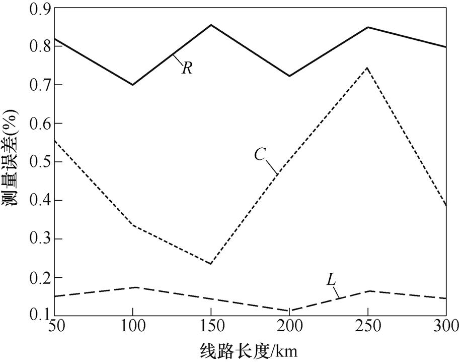
图8 本文方法在仅改变线路长度l2时的测量误差
Fig.8 The measurement error of the proposed method when only change the line length l2
不同电压等级的四回输电线路具有不同的零序分布参数,本文通过改变仿真模型的大地电阻率及导线的半径来改变线路初始的零序分布参数。以表2中的理论值为基准,假设线路分布参数偏离该基准值,得到的仿真测量结果如图9所示。
从图9给出的相对误差数据来看,在零序分布参数理论值偏离基准值较大的范围时,本文方法的测量误差仍然保持在较小的数值。本文方法通过严谨的数学推导,并未对理论初值进行限定,因此具备很好的鲁棒性,可适用于任意电压等级的四回非全线平行输电线路。
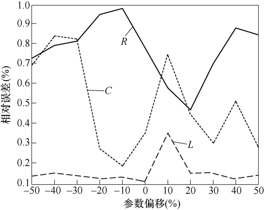
图9 零序分布参数偏离基准值时本文方法的测量精度
Fig.9 The measurement accuracy of the proposed method when zero sequence distributed parameters deviate from the reference values
本文提出了一种四回非全线平行输电线路零序分布参数精确测量方法,根据理论推导和仿真结果得到以下结论:
1)传统测量方法采用集中参数模型,在长距离输电线路中受线路分布效应的影响,且认为线路c与线路d两部分的参数相等,其零序参数的测量精度明显不足;现有方法因其适用范围的局限性,所能测量的零序分布参数较少,且对零序电容的测量误差较大;本文方法基于分布参数模型,单独处理四回耦合部分和双回耦合部分,采用逻辑缜密的数学推导公式,得到零序分布参数的精确解析解,故具有很高的测量精度。
2)由于四回输电线路架设形式的对称性,本文方法所需的测量方式减少为四种,这与需要12种测量方式的传统方法相比,显著提高了测量效率,且本文方法能够同时求得四回非全线平行输电线路的24个零序参数。
3)本文方法对线路长度的变化具有很强的适应性,且测量精度不受零序参数理论初值的影响,故本文的测量方法可适用于任意电压等级的长距离四回非全线平行输电线路,同时也为四回非全线平行线路的其他布线形式提供了求解零序分布参数的 思路。
附 录
 元素表达式为


参考文献
[1] 李少岩, 任乙沛, 顾雪平, 等. 基于短路电流约束显式线性建模的输电网结构优化[J]. 电工技术学报, 2020, 35(15): 3292-3302.
Li Shaoyan, Ren Yipei, Gu Xueping, et al. Opti- mization of transmission network structure based on explicit linear modeling of short circuit current constraints[J]. Transactions of China Electrotechnical Society, 2020, 35(15): 3292-3302.
[2] 龚仁敏, 刘宇, 王德林, 等. 一种混压同塔四回线路跨电压故障的通用计算方法[J]. 电力系统自动化, 2019, 43(12): 172-179.
Gong Renmin, Liu Yu, Wang Delin, et al. A general calculation method for cross-voltage fault on mixed- voltage four-circuit line on the same tower[J]. Auto- mation of Electric Power Systems, 2019, 43(12): 172-179.
[3] 陈玉, 文明浩, 王祯, 等. 基于低频电气量的超高压交流线路出口故障快速保护[J]. 电工技术学报, 2020, 35(11): 2415-2426.
Chen Yu, Wen Minghao, Wang Zhen, et al. A high speed protection scheme for outgoing line fault of HVAC transmission lines based on low frequency components[J]. Transactions of China Electrotech- nical Society, 2020, 35(11): 2415-2426.
[4] 郑涛, 吴丹, 张嘉琴, 等. 混压同塔四回线强电弱磁系统跨电压不接地故障短路计算[J]. 电力系统自动化, 2017, 41(15): 155-161.
Zheng Tao, Wu Dan, Zhang Jiaqin, et al. Short-circuit calculation of cross-voltage unearthed fault in strong- electric and weak-magnetic system of mixed-voltage four-circuit lines on the same tower[J]. Automation of Electric Power Systems, 2017, 41(15): 155-161.
[5] 贾科, 赵其娟, 冯涛, 等. 柔性直流配电系统高频突变量距离保护[J]. 电工技术学报, 2020, 35(2): 383-394.
Jia Ke, Zhao Qijuan, Feng Tao, et al. High-frequency fault component distance protection for flexible DC distribution system[J]. Transactions of China Electro- technical Society, 2020, 35(2): 383-394.
[6] 刘树鑫, 卓裕, 李津, 等. 基于微型同步相量单元数据的配电线路故障测距方法[J]. 电气技术, 2020, 21(10): 63-70.
Liu Shuxin, Zhuo Yu, Li Jin, et al. Distribution line fault location method based on micro-synchronous phasor unit data[J]. Electrical Technology, 2020, 21(10): 63-70.
[7] Eduardo C M C, Sergio K. Estimation of transmission line parameters using multiple methods[J]. Generation Transmission & Distribution Iet, 2015, 9(16): 2617- 2624.
[8] Wang Yang, Xu W. Algorithms and field experiences for estimating transmission line parameters based on fault record data[J]. IET Generation Transmission & Distri- bution, 2015, 9(13): 1773-1781.
[9] 倪识远, 胡志坚, 傅晨宇. 单回不对称输电线路分布参数的测量方法[J]. 电工技术学报, 2018, 33(5): 1086-1095.
Ni Shiyuan, Hu Zhijian, Fu Chenyu. A method for measuring the distributed parameters of single-circuit asymmetric transmission line[J]. Transactions of China Electrotechnical Society, 2018, 33(5): 1086-1095.
[10] 刘欣, 黄少锋, 张鹏, 等. 混压同塔线路跨电压不接地短路时低压系统过电压计算[J]. 电力自动化设备, 2018, 38(1): 116-120.
Liu Xin, Huang Shaofeng, Zhang Peng, et al. Over- voltage calculation of low-voltage system for mixed- voltage on same tower transmission lines under unearthed cross-voltage fault[J]. Electric Power Auto- mation Equipment, 2018, 38(1): 116-120.
[11] 刘云鹏, 黄世龙, 陈思佳, 等. 同塔四回750kV六层横担输电线路电晕损失研究[J]. 高电压技术, 2019, 45(4): 1118-1123.
Liu Yunpeng, Huang Shilong, Chen Sijia, et al. Corona loss of 750kV four-circuit lines with six-layer cross-arms on the same tower[J]. High Voltage Tech- nology, 2019, 45(4): 1118-1123.
[12] Halim S A, Bakar A H A, Illias H A, et al. Lightning back flashover tripping patterns on a 275/132kV quadruple circuit transmission line in Malaysia[J]. IET Science Measurement Technology, 2016, 10(4): 344-354.
[13] 黄学良, 王瑜, 闻枫. 1000kV/500kV同杆混压四回输电线路电磁环境影响因素及优化措施分析[J]. 高电压技术, 2015, 41(11): 3642-3650.
Huang Xueliang, Wang Yu, Wen Feng. Electro- magnetic environment influence factors of quadruple- circuit transmission line with 1000kV/500kV dual voltage on the same tower and optimization measures analysis[J]. High Voltage Technology, 2015, 41(11): 3642-3650.
[14] 李建明, 朱康. 高压电气设备试验方法[M]. 2版. 北京: 中国电力出版社, 2001.
[15] 梁志瑞, 牛胜锁, 靳楠. 交流输电线路参数测量现状及发展趋势[J]. 电力系统自动化, 2017, 41(11): 181-191.
Liang Zhirui, Niu Shengsuo, Jin Nan. Current status and development trend of AC transmission line parameter measurement[J]. Automation of Electric Power Systems, 2017, 41(11): 181-191.
[16] Hu Zhijian, Xiong Min, Shang Haozhi, et al. Anti- interference measurement methods of the coupled transmission-line capacitance parameters based on the harmonic components[J]. IEEE Transactions on Power Delivery, 2016, 31(6): 2464-2472.
[17] Dasgupta K, Soman S A. Estimation of zero sequence parameters of mutually coupled transmission lines from synchrophasor measurements[J]. IET Generation, Transmission & Distribution, 2017, 11(14): 3539-3547.
[18] 肖遥, 邓军, 范毅, 等. 同塔四回交流输电线路零序参数的解耦测量[J]. 南方电网技术, 2016, 10(1): 54-59.
Xiao Yao, Deng Jun, Fan Yi, et al. Decoupling measurement of zero sequence parameters for four- circuit AC transmission lines on same tower[J]. Southern Power System Technology, 2016, 10(1): 54-59.
[19] 邓军, 肖遥, 郝艳捧. 新型同塔双回高压直流输电线路分布参数测量方法及工程应用[J]. 电力自动化设备, 2016, 36(3): 154-158.
Deng Jun, Xiao Yao, Hao Yanpeng. Measuring of distributed parameter and its application for dual-loop HVDC transmission lines on same tower[J]. Electric Power Automation Equipment, 2016, 36(3): 154-158.
[20] 胡志坚, 倪识远. 同塔四回线路分布参数的测量[J]. 电工技术学报, 2018, 33(3): 563-572.
Hu Zhijian, Ni Shiyuan. A new approach to measure the distributed parameters of quadruple-circuit trans- mission lines[J]. Transactions of China Electro- technical Society, 2018, 33(3): 563-572.
[21] 倪识远, 胡志坚, 杨安琪, 等. 混压同塔四回输电线路零序参数测量方法[J]. 电工技术学报, 2018, 33(11): 2468-2478.
Ni Shiyuan, Hu Zhijian, Yang Anqi, et al. An approach for measuring the zero sequence parameters of mix-voltage quadruple-circuit transmission lines on one tower[J]. Transactions of China Electrotechnical Society, 2018, 33(11): 2468-2478.
[22] 于仲安, 毕俊强, 郭培育, 等. 同塔四回输电线路故障选线新方案[J]. 电力自动化设备, 2019, 39(11): 127-132.
Yu Zhongan, Bi Junqiang, Guo Peiyu, et al. New fault line selection scheme for four-circuit transmission lines on same tower[J]. Electric Power Automation Equipment, 2019, 39(11): 127-132.
[23] 胡志坚, 熊敏, 李岩. 超高压同塔四回交流/双回双极直流线路零序参数测量法: 中国, 2014101270258[P]. 2014.
[24] Asprou M, Kyriakides E, Albu M M. Uncertainty bounds of transmission line parameters estimated from synchronized measurements[J]. IEEE Transa- ctions on Instrumentation and Measurement, 2019, 68(8): 2808-2818.
A Method for Measuring the Zero Sequence Distributed Parameters of Quadruple-Circuit Non-Full-Line Parallel Transmission Lines
Abstract With the development of power systems, the transmission corridors are becoming narrower, and it is very common for quadruple-circuit lines to share a part of the corridor. There is no corresponding line distributed parameter measurement method. This paper proposes an accurate measurement method for the distribution parameters of quadruple-circuit non-full-line parallel lines, establishes a non-uniform transmission line model of quadruple-circuit non-full-line parallel lines, and obtains the transmission matrix of the quadruple-circuit lines completely through Laplace transform. In addition, the mathematical expressions between the line parameters and the voltages, currents of the heads and ends of the lines are obtained. The zero-sequence voltages and currents of the first end and last end of the quadruple-circuit non-full-line parallel lines are simultaneously measured under four independent measurement modes, and are substituted into the proposed calculation formulae to solve 24 zero-sequence distributed parameters. The accuracy of the proposed method is verified by PSCAD simulation software. Compared with the existing measurement methods, the simulation results show that the proposed method has higher measurement accuracy than the existing methods.
keywords:Quadruple-circuit non-full parallel lines, non-uniform transmission lines, zero sequence distributed parameters, Laplace transform, simultaneous measurement
DOI: 10.19595/j.cnki.1000-6753.tces.210108
中图分类号:TM72
高明鑫 男,1997年生,硕士研究生,研究方向为输配电线路参数测量。E-mail: mingxin_gao@whu.edu.cn
胡志坚 男,1969年生,博士,教授,博士生导师,研究方向为电力系统稳定分析与控制、输电线路参数带电测量等。E-mail: zhijian_hu@163.com(通信作者)
收稿日期 2021-01-21
改稿日期 2021-05-24
国家自然科学基金资助项目(51977156)。
(编辑 陈 诚)