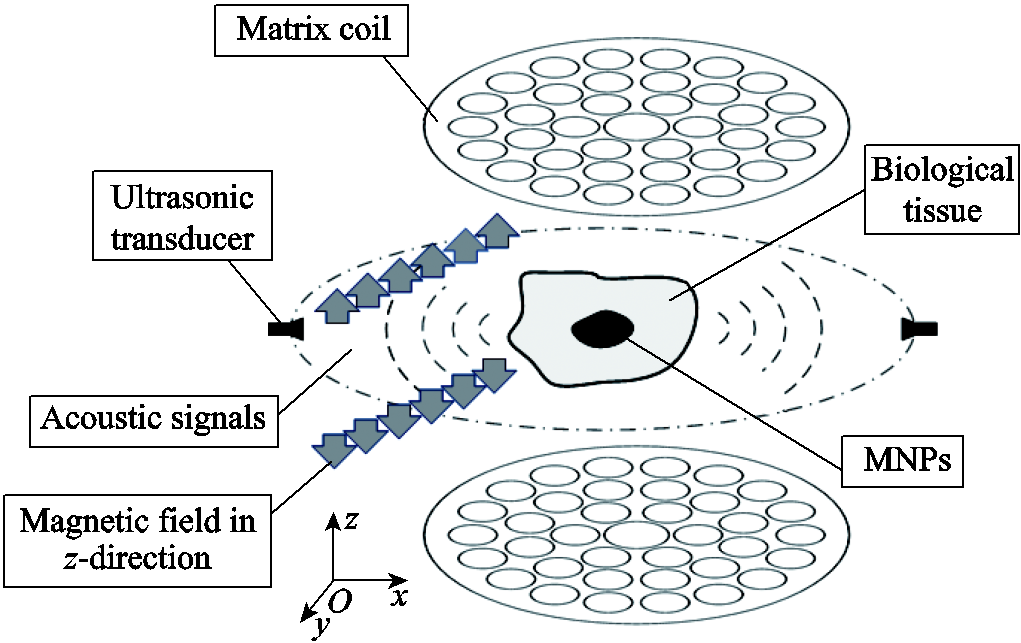
Fig.1 Principle of MACT-MI
Abstract Magnetoacoustic concentration tomography of magnetic nanoparticles (MNPs) with magnetic induction (MACT-MI) is a new method for MNPs concentration tomography. To reduce the amplitude of the excitation current source and produce a more stable magnetoacoustic signal, MACT-MI system based on matrix coils was studied. Optimal design of matrix coils used the artificial fish swarm algorithm based on beetle antennae search algorithm (BAS-AFSA). According to the optimization results the physical process of MACT-MI was solved by using COMSOL and then the results were compared with the results of Maxwell coils. A concentration gradient model was also constructed based on the distribution of MNPs in the actual biological tissue environment, and both the magnetic force and sound pressure distribution in the region of interest (ROI) were obtained. The results show that the matrix coils designed in this paper can produce a more stable sound pressure signal and a more uniformly distributed gradient magnetic field with equal size under a smaller excitation. According to the constructed concentration gradient model, both the magnetic force and the width of the sound pressure wave of MNPs are proportional to the width of the gradient region, and the peak value of sound pressure is proportional to the concentration gradient in the gradient region. The results provide a prospective basis for the design of imaging equipment, the follow-up experiments and clinical applications of MACT-MI.
Keywords:Magnetic nanoparticles with magnetic induction (MACT-MI), artificial fish swarm algorithm based on beetle antennae search algorithm, matrix coils, concentration gradient, magnetic force, sound pressure
Magnetoacoustic concentration tomography of magnetic nanoparticles (MNPs) with magnetic induction (MACT-MI) is a method for imaging the concentration of MNPs with the aid of inductive magnetoacoustic imaging technology, by measuring the acoustic signal generated by MNPs in the time-varying magnetic field to reconstruct the image of the concentration of MNPs. It naturally overcomes the problem of electromagnetic interference between the driving and detecting coils and combines the advantages of electromagnetic technology and ultrasound technology. With the advantages of non-invasive, good contrast, high sensitivity and spatial resolution, which is expected to further improve the imaging resolution, MACT-MI provides a basis for tumor therapy and quantitative detection of MNPs. Currently, the gradient magnetic field excitation unit of the MACT-MI is a Maxwell coil[1]. In order to let the ultrasound probe sense the magnetoacoustic signal, the radius of the Maxwell coil needs to be at least 0.8m and a current of approximately 200A is required, which is a great challenge for the heat dissipation of the gradient coil. Therefore, it is necessary to explore a gradient magnetic field implementation method for the MACT-MI, which can solve the problem of high excitation current and heat dissipation difficulties of the MACT-MI.
Matrix gradient coils can compensate for the shortcomings of conventional coils by applying different pulse sequences to produce simple or complex magnetic fields[2]. In 2010, C. Juchem et al. first proposed a gradient coil system consisting of 24 circular coils, demonstrating both theoretically and experimentally that the system is capable of generating highly complex magnetic fields in a fairly flexible manner[3]. In 2011, the multi-coil system was divided into top and bottom parts to eliminate the uneven magnetic field in the region of interest (ROI)[4]. In 2014, P. T. While et al. proposed a method for the design of irregular multi-coil systems and compared it with the gradient coil system proposed by C. Juchem, theoretically demonstrating that the system offers significant improvements in accuracy and efficiency[5]. In 2016, Jia Feng et al. referred to this type of gradient coil system as a matrix gradient system and proposed a new measurement method for matrix coil performance[6]. In 2018, Xu Yajie et al. used the matrix coil technique to homogenize the field of Halbach magnets. The research showed that the matrix coil can effectively generate the target magnetic field of all orders and can be applied to miniaturized magnetic resonance systems based on Halbach magnets[7]. In 2019, Wang Qiang et al. used a combination of particle swarm algorithm and genetic algorithm to optimize the design of matrix coils. The results showed that the matrix coils designed by this method have good linearity and meet the requirements of magnetic resonance imaging (MRI)[8]. In 2020, A. Aghaeifar et al. optimized the angle, axial position and coil size of 32 rectangular coils to improve the uniformity of gradient magnetic field in the ROI without increasing the number of local coils[9]. All of the above studies have shown that matrix gradient coils are very flexible. And compared to the larger current and heat dissipation conditions required by Maxwell coils, matrix gradient coils are safer and more suitable for various environments.
In this paper, in order to reduce the MACT-MI excitation current and improve the stability of the sound pressure signal, the gradient magnetic field excitation unit is changed from the Maxwell coils to the matrix coils designed by the artificial fish swarm algorithm based on beetle antennae search algorithm (BAS-AFSA). The current of excitation is greatly reduced, and a gradient magnetic field with higher uniformity is generated. Meanwhile, the concentration gradient model of the imaging target is established, and the changing law of MNPs magnetic force and sound pressure under the condition of concentration gradient is studied.
As is shown in Fig.1, in MACT-MI, MNPs are injected into biological tissues, and a time-varying magnetic field in z-direction generated by a matrix coil is applied. The magnetized MNPs vibrate magnetically in interaction with the time-varying magnetic field and produce an acoustic wave.
Fig.1 Principle of MACT-MI
The different concentrations of MNPs in biological tissues lead to the result that different magnetic forces act on MNPs, which further leads to different sound pressures. The sound pressure signal containing the concentration information is detected by the rotating ultrasonic transducer. Based on the nonlinear relationship between the sound pressure and the concentration of MNPs, the images of the MNPs concentration distribution were reconstructed by the time reversal method and the finite difference method.
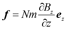
In MACT-MI, the sound source provided by time-varying magnetic force makes MNPs vibration create ultrasonic signals. With the application of a z-direction external gradient magnetic field, the magnetic force f is described as [10]
 (1)
(1)
where N is the number of MNPs per unit volume; m is the magnitude of the magnetic moment; ez is the unit vector in z-direction; and  is the gradient magnetic field in z-direction. The magnitude of the magnetic force is determined by the product of the concentration of MNPs and the gradient of the external magnetic field. And matrix coils can produce a more uniform gradient magnetic field at smaller excitation, which is effective for improving the imaging quality and simplifying the heat dissipation condition. Previous studies have shown that in order to produce a sound pressure level that can be measured by an ultrasonic transducer, the gradient magnetic field for MACT-MI needs to reach about 0.1T/m[10].
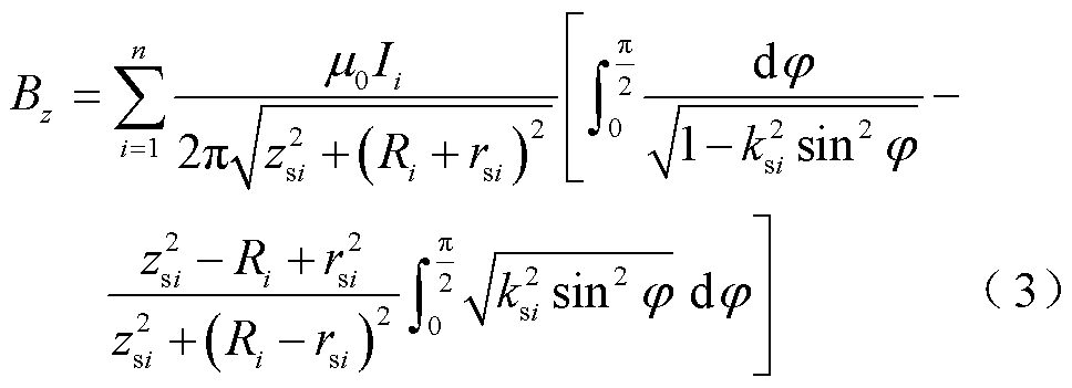
The matrix gradient coil consists of several circular coils and the Biot-Savart law is the basic formula for studying the magnetic fields generated by these coils. By combining the Biot-Savart law with the MACT-MI theory, the z-component of the magnetic flux density generated by a single current-carrying circular coil at any point Q(ρ, θ, z) can be derived analytically[11].
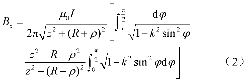
where I is the coil current; μ0 is the vacuum permeability; R is radius of the coils; z and ρ are the coordinates in cylindrical coordinate system; 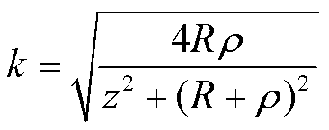 is the quantity determined by ρ, z and R; and φ is the integral item of the elliptic integral.
According to the superposition theorem of magnetic field, the z-components of the magnetic flux density produced by multiple circular coils are superimposed. The magnetic field generated by the matrix coil at any point can be obtained as
where (ρsi, θsi, zsi) is the coordinate of any point in a columnar coordinate system with the center of the ROI as the coordinate origin and can be described as
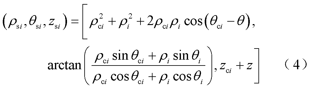
where (ρci, θci, zci) is the coordinates of the center of the ith coil, and ρi, θi and zi are the coordinates in the columnar coordinate system established with the center of the ith coil as the origin.
The value of the gradient magnetic field in the ROI is
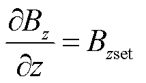 (5)
(5)
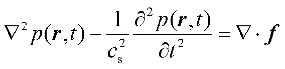
where Bzset is the gradient magnetic field in the ROI. Therefore, by adjusting the current and spatial position of the matrix coil, the gradient magnetic field generated by the matrix coil in the ROI can be modified, and a uniform gradient field is obtained ultimately. In the MACT-MI with a matrix coil as a gradient magnetic field system, the wave equation of active linear sound pressure is still applicable, and the equation can be expressed as[12]
 (6)
(6)
where r is any point in unbounded space; p(r, t) is the temporal and spatial distribution of sound pressure;  is the velocity of sound in biological tissues; and the divergence of magnetic force
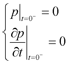
 is the sound source term. With the moment right before the matrix coils are electrified as the initial moment, there’s no gradient magnetic field in ROI. Then is 0. No magnetic force acts on MNPs and no sound source exists, so the initial conditions can be considered as
 (7)
(7)
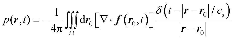
Combine Green's function in unbonded space with the convolution property to solve Equ.(6), the analytical solution of the unbonded sound field is obtained and the formula is shown in Equ.(8).
 (8)
(8)
where,  is the position of the source point; Ω is the space integral region; δ(·) is the impulse function.
The structural parameters of the matrix gradient coil should be set according to the ROI of the MACT-MI. Currently, the ROI of the MACT-MI is a cylinder with a base radius of 25mm and a height of 50mm[10]. In this paper, in order to ensure the uniformity of the gradient magnetic field in the ROI, the size of the matrix coil and the computational complexity are considered during the matrix coil design.
This article uses a matrix coil with a classic structure. It is made of multiple turns of wire, distributed on the surface of a cylinder or a plane. Compared with the larger current and higher heat dissipation condition required by traditional coils, matrix gradient coils are safer and more suitable for various environments. According to the Ref.[13], establish the matrix coil shown in Fig.2. The distance between the top and the bottom plates is 220mm, and the radius of each coil is 40mm.
In the preliminary study, it was found that under the same excitation conditions as the Maxwell coil, no matter how the coil radius changes, the magnetic field generated in the study area is smaller than the Maxwell coil. Therefore, it cannot reduce the excitation current and simplify the heat dissipation conditions. Under the same current excitation, the magnetic fields in ROI generated by the Maxwell coil and the matrix coil shown in Fig.2 are shown in Fig.3, where the radius of the Maxwell coil is 100mm.

Fig.2 Matrix coil
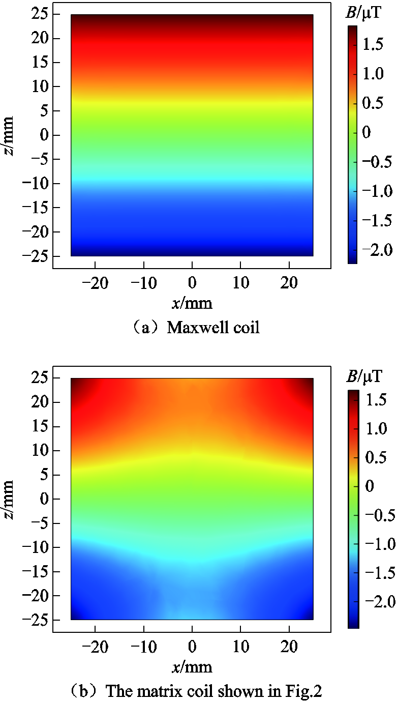
Fig.3 Magnetic field generated in the study area
The study found under the same excitation conditions, when the coil is closer to the study area, its contribution to the magnetic field is bigger. However, the matrix coil of the above structure does not have a corresponding coil directly above the study area, leading to a generated magnetic field smaller than the field generated by Maxwell coils in the study area under the same excitation.
Therefore, a new matrix coil structure shown in Fig.4 is established. The distance between the top and the bottom pole plates of the coil is 220mm, and the radius of each coil is 40mm. Under the same excitation conditions, the magnetic field generated in ROI is shown in Fig.5. The magnetic field is significantly larger than the field generated by Maxwell coils, which reduces the excitation current and simplifies the heat dissipation conditions.

Fig.4 A new matrix coil structure
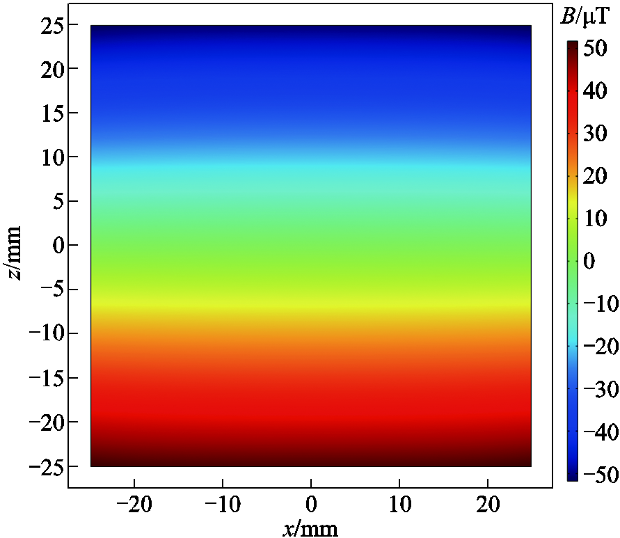
Fig.5 Magnetic fields generated in ROI by new matrix coil structure
Through simulation, it is found that under the same excitation conditions, the uniformity of the gradient magnetic field in the ROI increases as the coil radius increases, while the intensity of the gradient magnetic field decreases. In addition, the uniformity of the gradient magnetic field in the study area will be higher when more coils exsit, but the calculation will be more complex. And the coils will need bigger excitation to play a regulatory role when they are far away from the study area. In order to ensure uniformity while reducing the amount of calculation, the number of coils in the gradient magnetic field excitation system is 74. The top and the bottom pole plates are respectively 37 circular coils of the same material. The coils of top and bottom pole plates are arranged on the same surface to reduce the mutual influence[14], and they are divided into four groups from the inside to the outside. Each group of coils carries the same current in the same direction. The coil closer to the ROI contributes the most to the magnetic field. In order to ensure the uniformity of the gradient magnetic field in the imaging area and reduce the excitation current, the center coil is set as a circular coil with an outer radius of 40mm and an inner radius of 32mm. The other coils are all set to an outer radius of 30mm and an inner radius of 22mm. The center distance between the top and bottom plates is set to d. The coils in top and bottom plates are electrified with currents of equal intensity and opposite directions; 37 pairs of circular coils are made of copper enameled wires of 2mm in diameter. The number of coil winding layers is 4; the number of turns is 20; and the height of each coil is 10mm. The schematic diagram of matrix coil is shown in Fig.6.
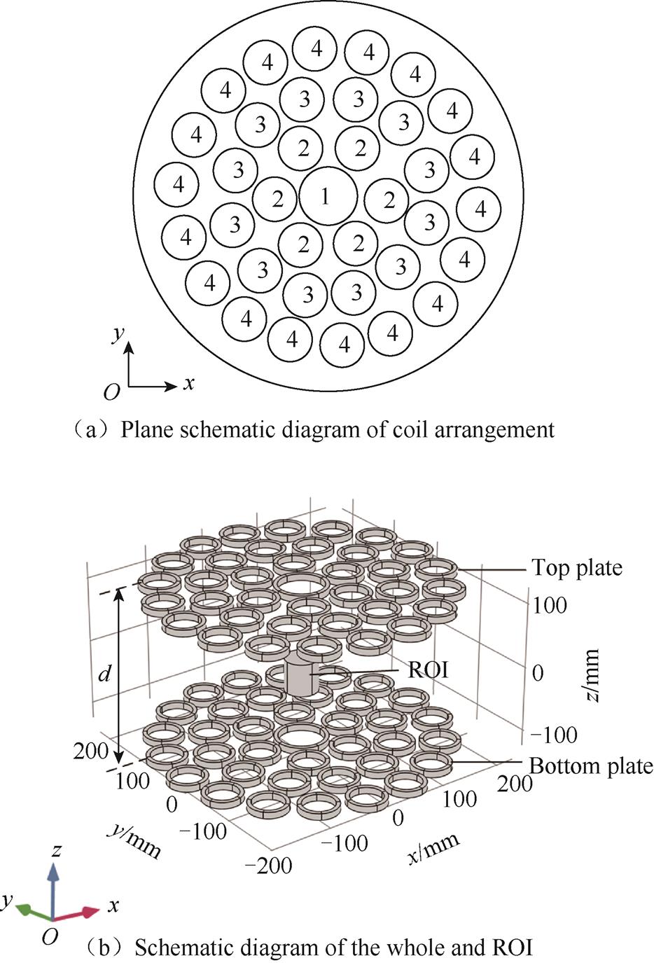
Fig.6 Schematic diagram of matrix coil
In this paper, BAS-AFSA[14-15] is used to optimize the design of the current values of the coils and the distance d of the top and bottom pole plates in the matrix gradient coil system with the assistance of COMSOL and Matlab software. The method is based on the beetle antennae search (BAS) algorithm to improve the speed of convergence and uses the artificial fish swarm algorithm (AFSA) to select the locally optimal individuals to avoid falling into the local optimum. In order to reduce the difficulty of modeling, the matrix coil is directly designed in the 3D magnetic field analysis module of COMSOL, and then the optimization algorithm is programmed in Matlab. Finally, the matrix coil is optimized using Matlab calling to COMSOL.
The current values of the four sets of coils and the distance d between the top and bottom pole plates are used as the centroid of the BAS. By sampling the points in the ROI and comparing the set value with the actual value, the fitness function is obtained as
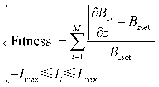 (9)
(9)
where Iiis the current of the ith set of coils;  is the target gradient; M is the total number of data points obtained; Imax is the set maximum current value; Bzi is the magnetic induction intensity in z direction at the ith data point. Since the imaging area of MACT-MI is axisymmetric, and the matrix coil designed in this paper is symmetrical along the imaging area, the paper collects only the uniform points for the xOz section. Taking a sampling point every 1mm, and 2 601 data points were adopted. The matrix coil of MACT-MI is designed by BAS-AFSA. The specific process of the algorithm is shown in Fig.7, and the specific steps are as follows:
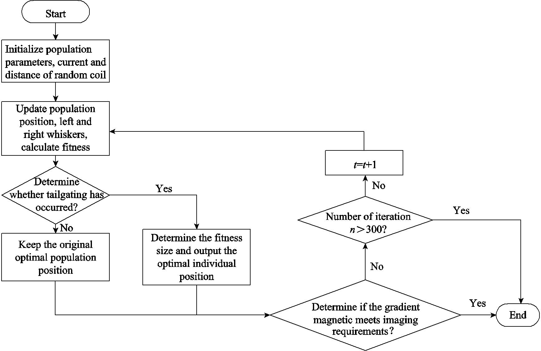
Fig.7 Flow chart of BAS-AFSA
1) Set the structure parameters of the matrix coil. Conduct modeling and simulation in COMSOL to obtain the magnetic field distribution in the study area without optimization. Where the initial currents of the coils and the initial distance between the top and bottom plates are I1=30A, I2=30A, I3=30A, I4=30A and d=100mm.
2) Initialization. The number of artificial fish is set as 20; the visual distance of artificial fish is 2 and the step length is 1. Initialize the centroid of beetle antennae and the direction vector
 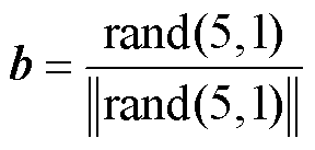 . The distance between the antennae and the step size is set as 1, the coefficient between the antennae and the step size is set as 5, the initial step size is set as 10, and the step attenuation factor is set as 0.95. The maximum number of iterations n is 300.
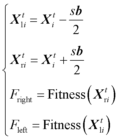
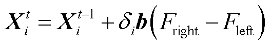
3) Use beetle antennae search algorithm to conduct iterative calculation. Each artificial fish is equivalent to a beetle, then the fitness and next position of the population are updated.
 (10)
(10)
 (11)
(11)
In 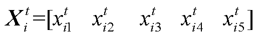 ,
,  represents the optimization value of the nth parameter of the ith beetle in the t iteration;
  ~
~ represent the current value of the first to the fourth group of coils, and
  represents the distance between the top and bottom plates;
  and
and  are the spatial positions of left and right antennae of beetle in the i iteration; s is the distance between the antennae of beetles; b is the direction vector of beetle antennae,
 is the attenuation factor of step size.
4) Update the position of beetle by using the rear-end idea of fish swarm algorithm as
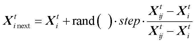 (12)
(12)
among the equation, rand( ) is the random function, uhich produces random number between 0 and 1; step is the step size, which is set to 1 here;  refers to the individuals in the population that are not too crowded and have the highest food concentration within the visual range.
5) If the current iteration times t is300 or the fitness is less than the set value, end the iteration process. If not, the number of iterations t equalsto t+1, then return to Step 3) to continue the iteration.
In this paper, BAS-AFSA is used to optimize the design of the matrix gradient coil system with the target gradient magnetic field of 0.1T/m. The variation of the fitness function with the number of iterations is shown in Fig.8. At the 42nd iteration, the fitness function is less than the set value, which ends the iteration. The optimized coil currents, structural parameters and the values of the fitness function are shown in Tab.1.
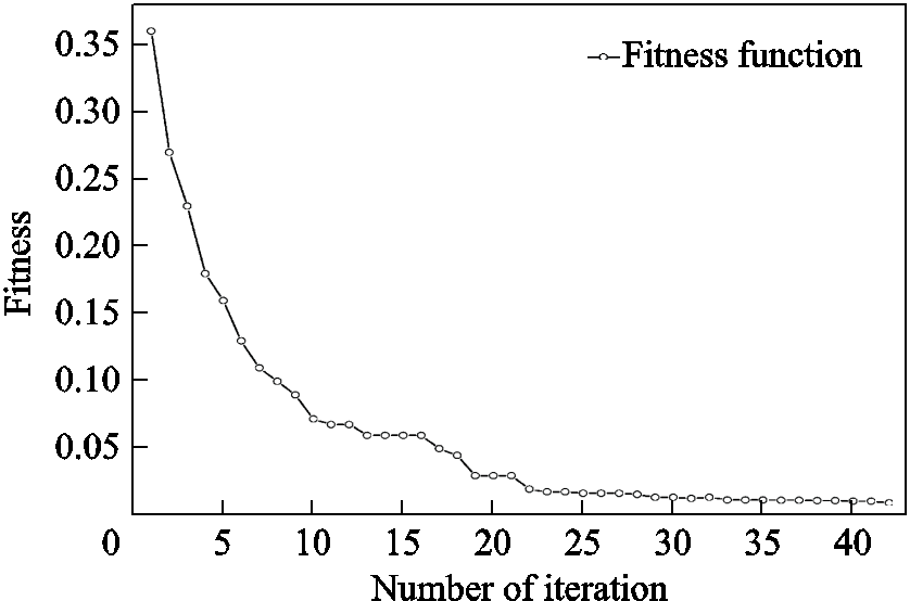
Fig.8 The change of fitness function with the number of iterations
Tab.1 Results of optimization
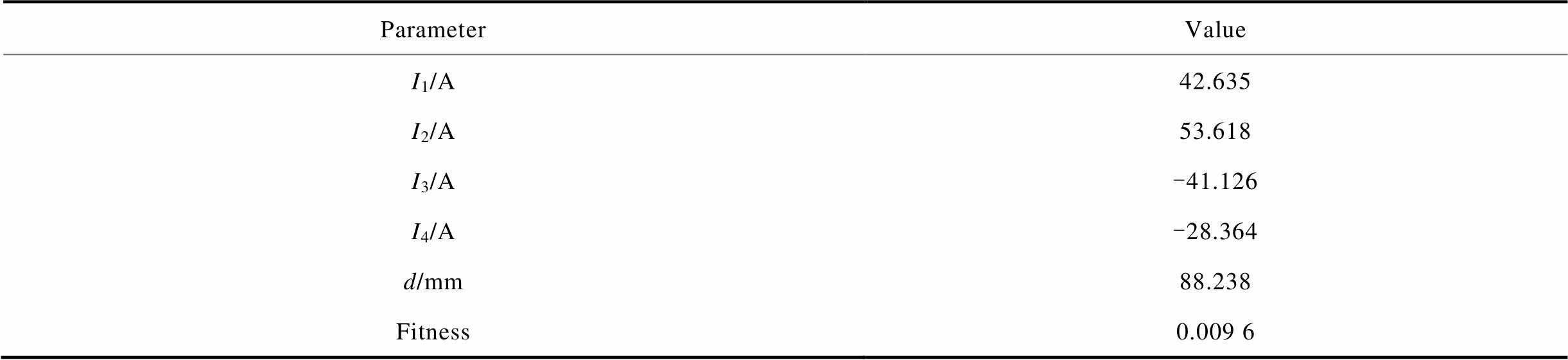
ParameterValue I1/A42.635 I2/A53.618 I3/A-41.126 I4/A-28.364 d/mm88.238 Fitness0.009 6
To compare the gradient magnetic field generated by the optimized matrix coil with the field generated by Maxwell coil in the ROI, the magnetic field analysis module of COMSOL software was used to calculate the results separately, as shown in Fig.9, where the excitation current in the Maxwell coil is 172.14A.

Fig.9 Gradient magnetic field in the ROI
The homogeneity of the gradient magnetic field is measured by the non-uniformity value δ[8].
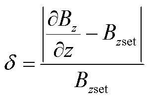 (13)
(13)
The magnetic field has the desired uniformity when δ is less than 1%, so the area where δ is less than 1% is set to be the area which meets the demand of MACT-MI. The area where Maxwell coils and matrix coils meet the imaging requirements on the xOz section of the ROI is shown in Fig.10. The area where the Maxwell coil meets the MACT-MI demand in Fig.10a is significantly smaller than that of the optimally designed matrix gradient coil in Fig.10b.

Fig.10 Regions meeting MACT-MI imaging
Further, in order to study the law describing how the gradient magnetic field variates with space. As shown in Fig.11, five section lines with the length of 60mm and the distance of 5mm from each other are taken as reference lines on the xOz cross section, and the variation curve of the gradient magnetic field with space position are plotted in Fig12. The uniformity of gradient magnetic field in the ROI of Maxwell coil in Fig.12a is significantly lower than that of matrix gradient coil system in Fig.12b.
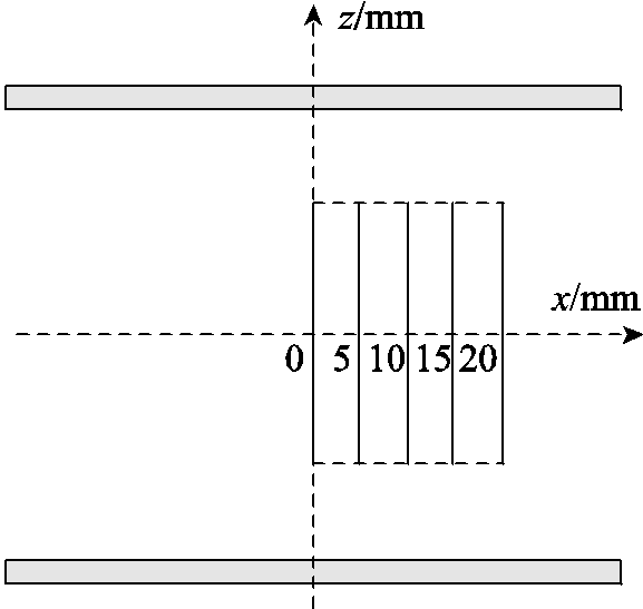
Fig.11 Schematic diagram of the position of the reference lines
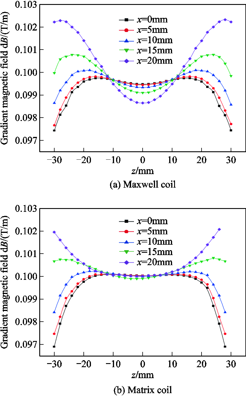
Fig.12 Gradient magnetic field distribution on the reference lines
Therefore, this paper uses the matrix gradient magnetic field system designed by the BAS-AFSA optimization algorithm. The uniformity of the region and gradient magnetic field meeting the imaging requirement is higher than the Maxwell coil. And the maximum current in all coils does not exceed 60A, which verifies the correctness and superiority of the matrix coil.
The average non-uniformity values and maximum non-uniformity values of Maxwell coils and matrix coils in the ROI by post-processing with COMSOL Multiphysics are shown in Tab.2. Therefore, the matrix gradient magnetic field system designed by BAS-AFSA is superior to Maxwell coils not only in the area size meeting the imaging requirements but also in gradient field uniformity. Even the maximum current in all coils is less than 60A.
Tab.2 The non-uniformity values of ROI
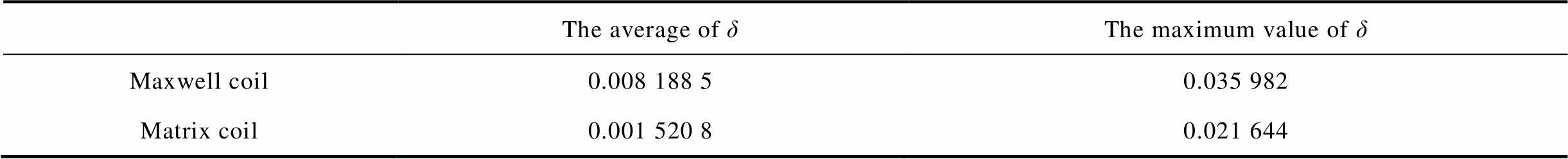
The average of δThe maximum value of δ Maxwell coil0.008 188 50.035 982 Matrix coil0.001 520 80.021 644
Similar to other imaging methods, the research on MACT-MI is also divided into two parts: the forward problem and the inverse problem. The so-called forward problem refers to that for some physical processes, if the internal parameters of the physical process are known, some observable variables of the system are determined according to the constraint law of the system and some specific conditions, and the opposite process is called the inverse problem[16-19].
To further study the physical process of the MACT-MI forward problem under the excitation of the matrix coil, the biological tissue model shown in Fig.13 is established and the MNPs are embedded inside this tissue. Transient solutions are performed for Maxwell coils and matrix coils to compare the magnetic force distribution of MNPs under the two gradient systems. In this model, a cylinder with a bottom radius of 25mm and a height of 50mm is used to simulate biological tissues, and the relative permeability is set to 1. The magnetic properties of the biological tissue can be neglected. And the sphere with a radius of 5mm is embedded in the cylinder to simulate the MNPs cluster. The parameters of MNPs are taken from the water-soluble superparamagnetic nanoparticles EMG304 (Ferrotec USA. Corporation), whose specifications are shown in Tab.3[10,20].
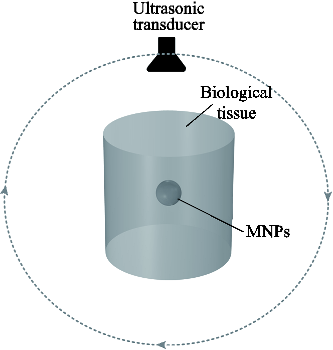
Fig.13 Biological tissue model
Tab.3 EMG 304 specifications
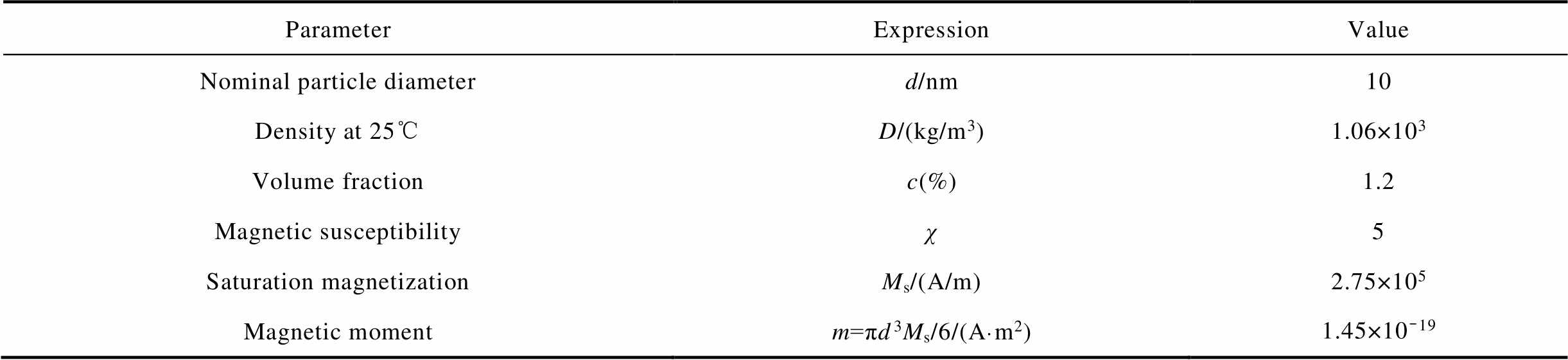
ParameterExpressionValue Nominal particle diameterd/nm10 Density at 25℃D/(kg/m3)1.06×103 Volume fractionc(%)1.2 Magnetic susceptibilityχ5 Saturation magnetizationMs/(A/m)2.75×105 Magnetic momentm=πd3Ms/6/(A·m2)1.45×10-19
When a matrix coil is used as a gradient field excitation system, the magnetic field in the ROI is generated by multiple pairs of coils, and when a Maxwell coil is used as a gradient field excitation system, the magnetic field in the ROI is generated by only one pair of coils. The pulse current which passes through the coil should satisfy that there is no reverse polarity oscillation when the current waveform drops to zero moment[21], so the excitation current is set as a sinusoidal attenuation truncation signal. The time characteristics of the incoming current of the Maxwell coil are shown in Fig.14a, and the time characteristics of the matrix coil current are shown in Fig.14b. Both currents reach a peak value near 0.2μs, and the duration is 2μs.
At present, the research on MACT-MI is carried out under the gradient magnetic field of 0.1~0.3T/m, and the current is linearly early correlated with the magnetic field. In order to ensure a certain margin, the peak current of the excitation current is valued 3.5 times of the optimization results.
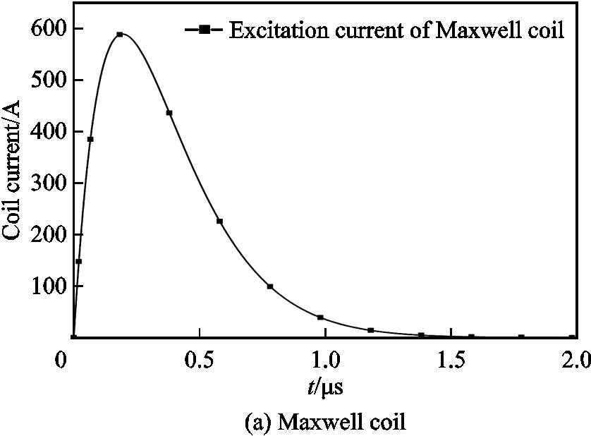
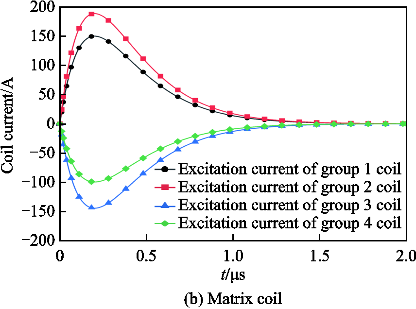
Fig.14 Excitation current of the coil
The concentration of MNPs is an important factor affecting the magnetism. If no limitation is applied, theoretically a higher concentration is better. While considering that applying condition of MACT-MI is in vivo experiments, the concentration of particles should not be too high in practical application. Kidney function can be seriously affected if the concentration of the particle solution is too high[22]. It is known from the paper that the iron content of EMG 304 solution has exceeded the iron content approved by the FDA[20], so it needs to be diluted during the experiment. The concentration of MNPs is set to 1×10¹⁵/mL in the simulation.
According to Equ.(1), the magnetic forces generated by Maxwell coils and matrix coils under pulsed current excitation were calculated using COMSOL Multiphysics. The results were shown in Fig.15.
As is shown in Fig.15, the magnetic force generated in the cluster region of MNPs at 0.5μs for both gradient magnetic field systems are concentrated on the biological tissue marked by MNPs and the values are approximately equal. This is because MNPs have a larger magnetization strength compared to biological tissues and are subjected to a larger magnetic force by the magnetic field, which provides the sound source for the sound field.

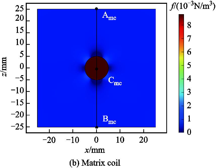
Fig.15 Comparison of magnetic forces
Further, to clearly observe the curves of the magnetic force on the MNPs with spatial position under the excitation of the two gradient magnetic field systems, the section line AB is taken in the model and the z-component curves of the magnetic flux density are plotted in Fig.16. The coordinates of the starting and ending points of the section line are (0mm, 0mm, -25mm) and (0mm, 0mm, 25mm), respectively. The results show that the magnetic force distribution in the ROI under the excitation of the two gradient magnetic field systems are approximately equal. However, the magnetic force of MNPs and nearby biological tissues is more uniform under the excitation of matrix coils, which can produce a more stable sound pressure signal and is more favorable for imaging. The magnetic force near the MNPs clusters in Fig.15a and Fig.15b appears partially distorted. This is due to setting the MNPs to a uniform concentration, and a sudden change occurs in concentration at the cluster boundaries, which in turn causes a distortion in the magnetic distribution.
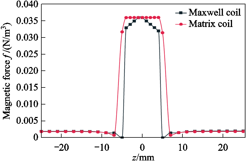
Fig.16 Magnetic force distribution along line AB
Considering the actual biological tissue environment, the concentration distribution of MNPs is gradually changing. Therefore, this paper established an MNPs concentration gradient model, and set the average concentration of MNPs in the concentration gradient model to be equal to the concentration in the uniform concentration model, which is
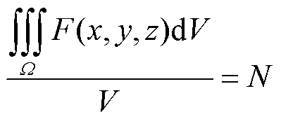 (14)
(14)
where N is the concentration of MNPs in the uniform concentration model; V is the volume of MNPs and F(x, y, z) is the concentration distribution function of MNPs in the concentration gradient model.
In the concentration gradient model, the concentration of MNPs varies along the radial direction, which can be expressed as
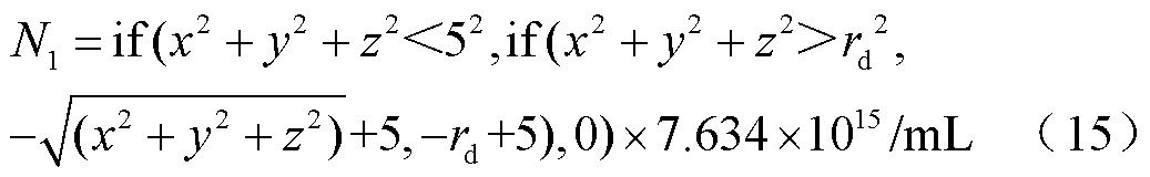
In the formula, x, y and z are coordinate components in cartesian coordinate system, and the unit is mm. The coefficient is 7.634×10¹⁵, which is due to the same average concentration of MNPs in the two models.
The distribution characteristics F(x, y, z) established in this paper on the xOz section are shown in Fig.17, which continuously changes in the spatial region set by the model. The average value is N and the width of the gradient region is rd.
The electromagnetic field is solved according to the concentration gradient model set by Equ.(15), and the magnetic force distribution in the ROI is shown in Fig.18. The magnetic force distribution near the MNPs cluster is uniform without obvious distortion, and the magnetic force presents a gradual distribution inside the cluster, which also conforms to the mathematical relationship revealed by Equ.(1).
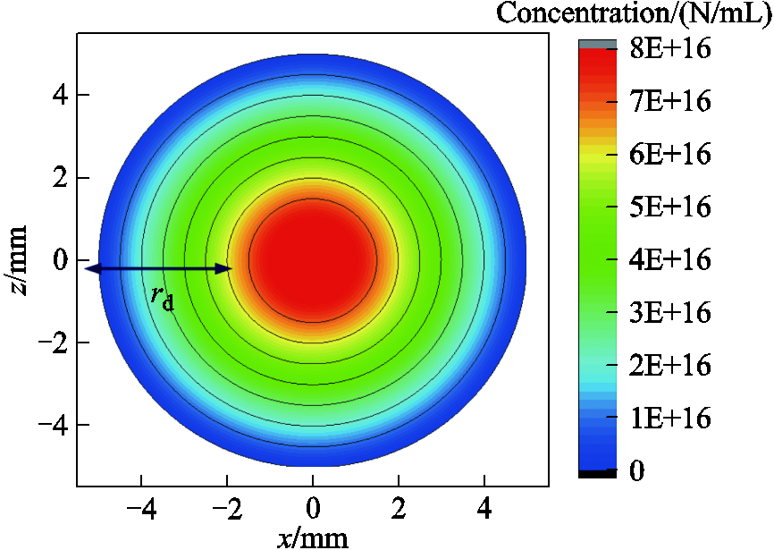
Fig.17 Concentration distribution of MNPs
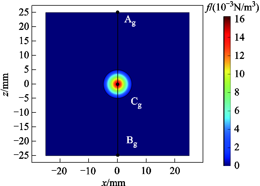
Fig.18 Magnetic force distribution of gradient concentration model in the ROI
In order to study the relationship between the magnetic force on MNPs and the width of the gradient region, the point Cg(0,0,0) in Fig.18 is taken as the observation point. According to the established concentration gradient model, in the spherical cluster of MNPs with a radius of 5mm, set rd to 0mm, 1mm, 2mm, 3mm, and 4mm, respectively, and calculate the trend of the magnetic force at this point over time and compare them. The change of magnetic force with width of gradient region is shown in Fig.19. As is shown in Fig.19, the magnetic force of MNPs is positively correlated with the width of the gradient region. This is because under the same conditions in which the average concentration MNPs are the same, the wider the gradient area is, the greater the MNPs concentration in the uniform area will be, and the magnetic force generated under the excitation of the external magnetic field will be bigger.
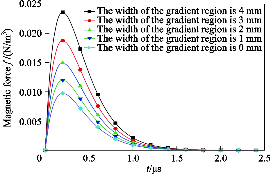
Fig.19 Change of magnetic force with width of gradient region
Based on the simulation results of the electromagnetic field part, the coupled solution of the established concentration gradient model is performed. And the solution is compared with the uniform concentration model. The sound pressure distributions of the two models are shown in Fig.20. Under the excitation of magnetic field in single z-direction, the sound pressure distribution of the uniform concentration model is more obviously different from that of the gradient concentration model. The sound pressure of the uniform concentration model is mainly concentrated at the top and bottom boundaries of the MNPs cluster. Due to the dipole source characteristics, the sound pressure equals in magnitude and opposites in direction. In addition, in the concentration gradient model, the sound pressure is not only distributed at the edge of the cluster, but also more uniformly distributed throughout the cluster. And the inner sound pressure in the cluster is slightly higher than the sound pressure at the boundary because the concentration of MNPs at the boundary is lower than the inner concentration.

Fig.20 Sound pressure distribution under different concentration models
Further, in order to study the changing law of the sound pressure with the width of the gradient region, according to the established concentration gradient model, the width of the gradient region is changed under the same condition of the average concentration. Take the section line EgFg as shown in Fig.20 and draw the sound pressure curve at t =1μs. The results are shown in Fig.21a, where the coordinates of the starting and ending points Eg and Fg of the line are (0mm, 0mm, 10mm) and (0mm, 0mm, -10mm) respectively. As the width of the concentration gradient region decreases, the distance between the sound pressure peaks is closer to the cluster diameter, and the sound pressure distribution in the cluster becomes more and more uneven. This is because the concentration of MNPs near the boundary region is gradually changing, which leads to the broadening of the sound pressure wave, and the center of wave is the center of the gradient region.
Furthermore, investigate the relationship between the sound pressure and the concentration gradient of the gradient model. With rd remaining the same as 3mm, change the density difference ΔN between the two ends of the gradient area and set ΔN to 1.0×10¹⁵mL, 1.5×10¹⁵mL, 2.0×10¹⁵mL, 2.5×10¹⁵mL and 3.0×10¹⁵mL, respectively. The sound pressure distribution along the line EgFg is calculated and the results are shown in Fig.21b. When rd is fixed, the peak of sound pressure gradually increases as the concentration difference in the gradient region increases. Because the peak sound pressure of the concentration gradient model is proportional to the concentration gradient in the gradient region in MACT-MI. In Fig.21a, with the decrease of rd, the peak sound pressure shows a trend of increasing and then decreasing, which is also due to the continuous change of the concentration gradient in the gradual area with the change of rd.
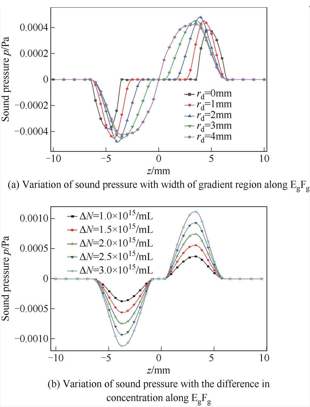
Fig.21 Variation of sound pressure
In order to reduce the excitation source amplitude and improve the stability of the sound pressure signal, a matrix coil suitable for MACT-MI is designed in this paper. The research is focused on the effects of the concentration gradient model of MNPs on the MACT-MI imaging process under matrix coils excitation. This paper includes the optimal design of matrix coils by BAS-AFSA, the variation of magnetic force in the ROI when using matrix coils as gradient magnetic field excitation units, and the interrelationship between magnetic force and sound pressure with different concentration gradient models. The main conclusions are as follows:
1) The matrix coil designed by BAS-AFSA has a wider ROI meeting the imaging requirements and the uniformity of the gradient magnetic field is also higher than that of the Maxwell coil. And the maximum current value in all coils does not exceed 60A. It is instructive for solving the problem of heat dissipation during the experiment.
2) The MNPs are subjected to more uniform magnetic force under the excitation of matrix coils, which can produce a more stable sound pressure signal and is more favorable to imaging.
3) Under the designed matrix coil excitation, the sound pressure is symmetrically distributed top and bottom along the magnetic field direction and in opposite directions. The sound pressure peak of the uniform concentration model appears at the boundary. While, the sound pressure peak of the gradient concentration model appears near the center of the gradient region. And the peak value of the sound pressure is proportional to the concentration difference between the two edges of the gradient region.
4) Under the condition of the same average concentration, the magnetic force is positively correlated with the width of the gradient region. The smaller width of the concentration gradient area is, the narrower the sound pressure waveform becomes. The distance between the sound pressure peaks gets closer to the cluster diameter and the sound pressure distribution in the cluster becomes more and more uneven.
Matrix coils method is a recently proposed new method for generating gradient magnetic fields, which can produce more uniform gradient fields with smaller excitation. This paper designed a matrix coil suitable for MACT-MI and proposed a concentration gradient model. Focused the research on the influence of the concentration gradient on the MACT-MI process under the excitation of the matrix coil, which makes the research of MACT-MI one step closer. Meanwhile, there is a lack of experiments to further investigate the magnetic field generated by the matrix coil and the magnetic force applied to the MNPs. At the same time, the inductance of the coil is not considered in the optimal design in this paper, and the algorithm needs further improvement. In addition, in the process of numerical calculation of sound source and sound pressure, this article assumes that the internal sound velocity of the human body is uniform, but in actual situations, the sound velocity in different tissues is generally not uniform, which also needs to be specifically considered in future research. In conclusion, this paper has done some in-depth research on MACT-MI and provided a basis for further experimental and clinical studies of the method.
References
[1] Shi Xiaoyu, Liu Guoqiang, Yan Xiaoheng, et al. Simulation research on magneto-acoustic concentration tomography of magnetic nanoparticles with magnetic induction[J]. Computers in Biology and Medicine, 2020, 119(9): 103653.
[2] He Hongyan, Wei Shufeng, Wang Huixian, et al. Matrix gradient coil: current research status and perspectives[J]. Chinese Journal of Magnetic Resonance, 2021, 38(1): 140-153.
[3] Juchem C, Nixon T W, McIntyre S, et al. Magnetic field modeling with a set of individual localized coils[J]. Journal of Magnetic Resonance, 2010, 204(2): 281-289.
[4] Juchem C, Nixon T W, McIntyre S, et al. Dynamic multi-coil shimming of the human brain at 7 T[J]. Journal of Magnetic Resonance, 2011, 212(2): 280-288.
[5] While P T, Korvink J G. Designing MR shim arrays with irregular coil geometry: theoretical considerations[J]. IEEE Transactions on Bio-Medical Engineering, 2014, 61(6): 1614-1620.
[6] Jia Feng, Schultz G, Testud F, et al. Performance evaluation of matrix gradient coils[J]. Magnetic Resonance Materials in Physics, Biology and Medicine, 2016, 29(1): 59-73.
[7] Xu Yajie, Yu Peng, Wu Zhenzhou, et al. Matrix coil (mc) active shimming research in halbach array magnet[C]//the 20th China Molecular Spectroscopy Annual Conferenc Abstract Collectione, Wenzhou, China, 2018: 326-327.
[8] Wang Qiang, Wei Shufeng, Wang Zheng, et al. Design of matrix gradient coils with particle swarm optimization and the genetic algorithm[J]. Chinese Journal of Magnetic Resonance, 2019, 36(4): 463-471.
[9] Aghaeifar A, Zhou Jiazheng, Heule R, et al. A 32-channel multi-coil setup optimized for human brain shimming at 9.4T[J]. Magnetic Resonance in Medicine, 2020, 83(2): 749-764.
[10] Yan Xiaoheng, Pan Ye, Chen Weihua, et al. Simulation research on the forward problem of magnetoacoustic concentration tomography for magnetic nanoparticles with magnetic induction in a saturation magnetization state[J]. Journal of Physics D: Applied Physics, 2021, 54(7): 075002.
[11] Zu Wanni, Ke Li, Du Qiang, et al. Electronically rotated field-free line generation for open bore magnetic particle tomography imaging[J]. Transactions of China Electrotechnical Society, 2020, 35(19): 4161-4170.
[12] Zhang Shuai, Li Zixiu, Zhang Xueying, et al. The simulation and experiment of magneto-motive ultrasound imaging based on time reversal method[J]. Transactions of China Electrotechnical Society, 2019, 34(16): 3303-3310.
[13] Chen Weijie, Chen Jie, Sun Huijun, et al. Simulation and analysis of irregular multicoil B0 shimming in C-type permanent magnets using genetic algorithm and simulated annealing[J]. Applied Magnetic Resonance, 2019, 50(1): 227-242.
[14] Zhou Lei, Dong Xueyu, Sun Fei. Economic dispatch of micro-grid based on improved artificial fish swarm algorithm[J]. Distribution & Utilization, 2019, 36(12): 62-68.
[15] Kroboth S, Layton K J, Jia Feng, et al. Optimization of coil element configurations for a matrix gradient coil[J]. IEEE Transactions on Medical Imaging, 2018, 37(1): 284-292.
[17] Zhao Yingge, Li Ying, Wang Lingyue, et al. The application of univariate dimension reduction method based on mean point expansion in the research of electrical impedance tomography uncertainty quantification[J]. Transactions of China Electrote-chnical Society,2021,36(18): 3776-3786.
[18] Liu Jing, Liu Guoqiang. Electrical particles imaging method and numerical study on the forward problem[J]. Transactions of China Electrotechnical Society, 2020, 35(22): 4621-4626.
[19] Li Xiaonan, Ren Wenting, Liu Guoqiang, et al. Preliminary conductivity reconstruction by high-resolution magnetic resonance electrical properties tomography for brain tumor diagnosis[J]. Transactions of China Electrotechnical Society, 2021, 36(18): 3860-3866.
[20] Hu Gang, He Bin. Magnetoacoustic imaging of magnetic iron oxide nanoparticles embedded in biological tissues with microsecond magnetic stimulation[J]. Applied Physics Letters, 2012, 100(1): 013704.
[21] Liu Guoqiang. Magnetoacoustic imaging technology[M]. Beijing: Science Press, 2014.
[22] Sun C, Lee J S H, Zhang Miqin. Magnetic nanoparticles in MR imaging and drug delivery[J]. Advanced Drug Delivery Reviews, 2008, 60(11): 1252-1265.
摘要 感应式磁声磁粒子浓度成像(MACT-MI)是一种基于磁声耦合效应的磁性纳米粒子(MNPs)浓度成像新方法,为降低激励源幅值,产生更加稳定的声压信号,该文提出一种基于矩阵式线圈的磁声磁粒子浓度成像系统,采用天牛须-鱼群优化算法对矩阵式线圈进行优化设计,根据优化结果采用多物理场仿真软件COMSOL对MACT-MI的物理过程进行求解,并将结果与Maxwell线圈进行对比,同时基于实际生物组织环境中的MNPs分布,构建浓度渐变模型,得到了成像区域的磁力、声压分布。结果表明,该文设计的矩阵式线圈能在较小的激励下产生大小相等且分布更为均匀的梯度磁场,从而产生更为稳定的声压信号;根据所构建的浓度渐变模型,MNPs所受磁力和声压波形宽度均与渐变区域宽度成正比,声压峰值与渐变区域的浓度梯度成正比。研究结果可为成像装备的设计以及MACT-MI的后续实验乃至临床应用提供研究基础。
关键词:磁声磁粒子浓度成像 天牛须-鱼群算法 矩阵式线圈 浓度渐变 磁力 声压
中图分类号:TM12
DOI: 10.19595/j.cnki.1000-6753.tces.210959
This work is partially supported bythe Natural Science Foundation of Liaoning Province (2019-ZD-0039) and the Basic Scientific Research Project of Liaoning Education Department(LJ2020JCL003).
Received June 30, 2021;
Revised January 22, 2022.
Note brief
Yan Xiaoheng, born in 1984, PhD, associate professor, research interests include electromagnetic detection and imaging.E-mail: xiaohengyan@163.com
Li Zhengxing, born in 1997, postgraduate, research interests include electromagnetic detection and imaging.E-mail: lizhengxing@163.com (Corres000ponding author)
(编辑 李冰)